Use of Fuzzy Cognitive Maps for Climate System Stability Analysis
Carlos Gay Garc
´
ıa and Iv
´
an Paz Ortiz
Programa de Investigaci
´
on en Cambio Clim
´
atico, Universidad Nacional Aut
´
onoma de M
´
exico, Mexico City, Mexico
Keywords:
Cognitive Maps, Climate System, Stability.
Abstract:
In the present work we use fuzzy cognitive maps for the qualitative analysis of the earth’s climate system dy-
namics. First of all, we identify the subsystems which determine, as a hole, the stability of the climatic system.
Later we develop cognitive maps (knowledge networks) based on the documented relationships between the
subsystems (nodes of the network). The relationships between the nodes can be precise (quantifiable) or fuzzy
(not quantifiable). Once the map is built, we use the state vector and adjacent matrix technique to assess the
response of the system (the system converges or diverges) to the changes in the input node values in order to
identify the possibles feedback. Then the Min-Max criteria is used to evaluate the effect of the network over
the nodes, according to the fuzzy weights assigned to the edges (causal relations between nodes). Finally, we
discuss some possible changes in the network in order to show how the system dynamic can be modified and
can lead the system into a desired equilibrium state.
1 INTRODUCTION
Fuzzy cognitive maps are fuzzy-graph structures for
representing causal reasoning between variable con-
cepts (Kosko, 1986). The concepts are represented
as nodes (C
1
,C
2
, ...,C
n
) in an interconnected network,
each node C
i
represents a concept and the edges e
i j
which connect C
i
and C
j
(denoted as C
i
→ C
j
) are
causal connections and express how much C
i
causes
C
j
. These edges can be negatives or positives. A posi-
tive relation C
i
→
+
C
j
states that if C
i
grows also does
C
j
, and a negative relation C
i
¯→ C
j
indicate that as C
i
grows C
j
decreases. The fuzzy cognitive maps have
been used to model different kind of systems, such
as control, social and economics systems, and also in
robotics, computed assisted learning, expert systems,
and many others. Even though cognitive maps have
been applied to many areas, little has been done in
atmospheric sciences. This is the importance of the
present work.
As an example of cognitive maps, consider the
following network of 4 nodes. Here we use posi-
tive (+) and negative (-) causality among the concepts.
The system state can be represented as a state vector,
which contains the values for each node at time t. For
example, the row vector v
0
= [1,0,0,0] at t
0
indicates
that only the first node in the system is ON at time
zero. As we said, the adjacent matrix of the network
expresses the causal relationships between nodes. In
Figure 1: 4-node network.
cognitive maps the adjacent matrix is always square.
In our example the matrix is:
M =



0 1 0 0
0 0 1 1
0 −1 0 −1
0 1 0 0



Then the system is iterated to get v for t
1
,t
2
, ...,t
n
. For
this, multiply the row vector by the matrix v ∗ M, so
we have:
v
n
= v
n−1
∗ M (1)
If we consider v
0
= [1,0,0,0], and the iterations are
made, we get:
v
1
= [0,1,0,0] The node I causes II.
511
Gay García C. and Paz Ortiz I..
Use of Fuzzy Cognitive Maps for Climate System Stability Analysis.
DOI: 10.5220/0004164205110517
In Proceedings of the 2nd International Conference on Simulation and Modeling Methodologies, Technologies and Applications (MSCCEC-2012), pages
511-517
ISBN: 978-989-8565-20-4
Copyright
c
 2012 SCITEPRESS (Science and Technology Publications, Lda.)

v
2
= [0,0,1,1] The node II light on the nodes III
and IV.
v
3
= [0,0,0,-1] The node III acts negatively over II
y IV, in the node II the negative effect vanishes.
v
4
= [0,-1,0,0] The node IV acts negatively on II.
v
5
= [0,0,-1,-1] Node II acts negatively over III y
IV.
v
6
= [0,0,0,1].
Finally, we obtain v
7
= [0,1,0,0], which is equal to
v
1
= [0,1,0,0]. In this case the system reaches a limit
cycle. In general it can be shown that for every ma-
trix the system converges to a point, to a limit cycle,
or diverges in the space of states for the system. If
we express the state vector as X(t) = (x
1
(t), ..., x
n
(t)),
and the signal value as S
i
, we define a threshold bi-
nary function, which limits the signal value by a pre-
defined threshold for each time t as:
S
i
(x
t
i
) =









1 si x
t
i
> U
i
S
i
(x
t−1
i
) si x
t
i
= U
i
0 si x
t
i
< U
i
(2)
In this way, the node values will be restricted be-
tween 0 and 1. Similarly, it can be defined ternary
functions with values of {-1,0,1}.
2 SUBSYSTEMS OF THE
CLIMATIC SYSTEM
The proposed subsystems to describe the dynamic
of the climatic system are based on the article “A
safe operating space for humanity” written by Johan
Rockstr
¨
om (2009), and also in the Intergovernmental
Panel on Climate Change Report (IPCC, 2007).
These are:
Industrialization.
This process comprises: social and economic devel-
opment, technology tendencies and its applications,
industry grown, as well as demographic changes
associated with these processes (IPCC, 2007).
Climate Change.
This concept refers to increase in the mean temper-
ature of the earth, i.e. changes in climate variability
in terms of the extreme and mean values. (IPCC,
2007). Specifically, we refer to antropogenic climate
change, which is a consequence of the human activity.
Changes in CO
2
Concentration.
Defined as the increase in the parts per million of
CO
2
molecules in the atmosphere (IPCC, 2007).
Biodiversity Loss.
Refers to the extinction rate, the number of species
loss per million per year. Mace and collaborators
(2005), define biodiversity as the variability of living
organisms, included terrestrial and marine ecosys-
tems, other aquatic ecosystems and the ecological
systems in which they reside. Comprises the diversity
within species, among species and within ecosystems.
Mace emphasizes three levels of biodiversity: genes,
species, and ecosystems. Biodiversity loss during
the industrial period has grown notably. The species
extinction rate is estimated against the fossil record.
The extinction rates per million per year varies for
marine life between 0.1 and 1 and for mammals
between 0.2 and 0.5.
Phosphorus and Nitrogen Cycles.
The changes in P and N cycles are estimated with
the quantity of P going to the oceans, measured in
million tones per year, and with the amount of N
2
removed from the atmosphere for human use, also in
million tones per year.
Ocean Acidification.
Defined as the ocean PH increase, mainly in the
surface layer. The acidification process is closely
related with the CO
2
emission level. When the
atmosphere CO
2
concentration increases, the amount
of carbon dioxide dissolved in water as carbonic acid
increases, which in turn, modifies the surface PH.
Normally, the ocean surface is basic with a PH of
approximately 8.2. Nevertheless, the observations
show a decline in PH to around a value of 8. These
estimations are made using the levels of aragonite
(a form of calcium carbonate) that is created in the
surface layer. This concept has an important relation
with biodiversity loss as many organisms (like corals
and phytoplankton), basic for the food chain, use
aragonite as to produce their skeletons or shells. As
the aragonite value decreases, the ocean ecosystems
weaken, and the fisheries production falls. (Foley et
al., 2010).
Land Use (Urban Growth and Agriculture
Use).
The IPCC defines the change in land use as the
percentage of global land converted into cropland.
A general definition of land use change includes
any type of human use. This transformation, either
to cropland or urban, increases the biodiversity
loss, which is associated with the destruction of
ecosystems. In order to establish the difference in
SIMULTECH2012-2ndInternationalConferenceonSimulationandModelingMethodologies,Technologiesand
Applications
512

land use between urban growth and agriculture use,
and their different consequences, we include both
concepts as nodes in the map.
Increase in Fresh Water Demand.
Defined as an increase in its current use. Today
around the globe the annual use of freshwater from
rivers, lakes and groundwater aquifers is of 2,600
km
3
. From that, 70% is destined for irrigation,
20% for industry, and 10% for domestic use. This
extraction causes the drying and reduction body
waters. (IPCC, 2007).
Stratospheric Ozone Depletion.
O
3
depletion is estimated according to the ozone
concentration in the atmosphere in Dobson Units.
1
Chemic Pollution.
It refers to the emitted quantity, persistence, or
concentration of organics pollutants, plastics, heavy
metals, chemical and nuclear residues, etc., which
affect the dynamic of ecosystems.
Aerosol Loading.
Referred as the concentration of particles in the
atmosphere. These can be lead, copper, magnesium,
iron, traces of fire, ashes, etc.
With the use of these definitions we create a cogni-
tive map establishing and weighting the relationships
among the concepts (different subsystems). Through
the analysis of the map we create a qualitative global
vision of the climatic system dynamics.
3 THE MODEL
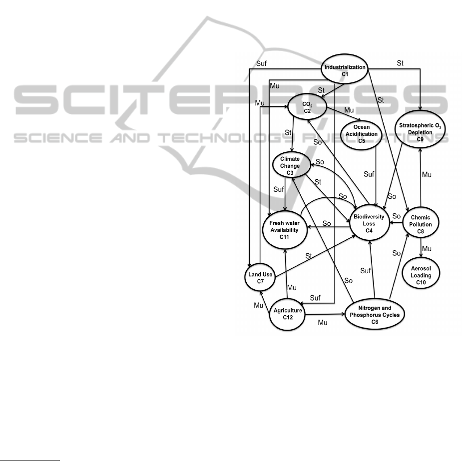
Using the subsystems we build the cognitive map
shown below. The nodes and the relations among
them are represented in it. These relations had been
established with the consulted references. As many
relations between concepts can not be quantifiable,
i.e. can not be expressed numerically, we have used
linguistic variables. These variables will be later
used with the Min-Max criteria. To analyze the
system we start with the adjacent matrix and the
state vector, considering values of 0 and 1 (positive
causality and no causality) and a binary function.
1
Dobson unit is a measure of the ozone layer thickness,
equal to 0,01 mm of thickness in normal conditions of pres-
sure and temperature (1 atm and 0 C respectively), express
as the molecule number. DU represents the existence of
2.69 x 10
16
molecules per square centimeter.
It is important to note that in the map all the rela-
tions (edges) are positives, so the associated matrix is:
M =
























0 1 0 0 0 0 1 1 1 0 1 1
0 0 1 0 1 0 0 0 0 0 0 0
0 0 0 1 0 0 0 0 0 0 1 0
0 1 1 0 0 0 0 0 0 0 1 0
0 0 0 1 0 0 0 0 0 0 0 0
0 0 1 1 0 0 0 1 0 0 0 0
0 1 0 1 0 0 0 0 0 0 0 0
0 0 0 1 0 0 0 0 1 1 0 0
0 0 0 1 0 0 0 0 0 0 0 0
0 0 0 0 0 0 0 0 0 0 0 0
0 0 0 1 0 0 0 0 0 0 0 0
0 0 0 0 0 1 1 0 0 0 1 0
























Figure 2: Cognitive map with fuzzy edges. We have used
four causal quantities: Strong (St), Much (Mu), Sufficient
(Suf), and, Some (So).
First we turn on the first node in the state vector
a
0
= [1, 0, 0, 0, 0, 0, 0, 0, 0, 0, 0, 0], then we iterate a ∗
M, and reset to 1 the first entrance of the vector a
after each iteration i.e. (a[1] = 1). In the network the
shortest way between the first node (C
1
) and any other
consists of two steps, so when we turn on the node C
1
the system converges to the equilibrium state “a
2
” in
two steps, with:
a
2
= [1, 1, 1, 1, 1, 1, 1, 1, 1, 1, 1, 1]
This vector state represents the increase of each node
UseofFuzzyCognitiveMapsforClimateSystemStabilityAnalysis
513

due to the causal action of C
1
but it does not say any-
thing more, i.e. the action of c
1
causally increases
the other nodes of the network when is forced with
(a[1] = 1). When the first node is not forced (a[1] = 1
only in t
0
), the system reaches an equilibrium among
the nodes which have feedback. In this case we get:
a
0
= [1, 0, 0, 0, 0, 0, 0, 0, 0, 0, 0]
a
1
= [0, 1, 0, 0, 0, 0, 1, 1, 1, 0, 1, 1]
The nodes that are connected with C
1
turn on.
a
2
= [0, 1, 1, 1, 1, 1, 1, 0, 1, 1, 1, 0]
The nodes 3, 4, 5, 6, 10 and 11 turn on. These are
the nodes connected in two steps with C
1
. While
node 8 turn off (no node activates it in this iteration).
In the fifth iteration the system converges to vector a
5
:
a
5
= [0, 1, 1, 1, 1, 0, 0, 0, 0, 0, 1, 0]
Another approximation is to start the first node
with an intermediate value in [0, 1], which repre-
sents the case where the industrialization node de-
creases from the current level but is not zero. In
this case we choose the value 0.5 i.e. assuming
an intermediate industrialization activity. We first
iterate the system turning on the first node after
each iteration. In the following experiment we start
the system without turning on the node. In the
first case, the system converges in six iterations to
a
6
= [0, 1, 1, 1, 1, 0, 0, 0, 0, 0, 1, 0], and in the second
case the system converges in four iterations to a
4
=
[0.5, 1, 1, 1, 1, 0.5, 1, 1, 1, 1, 1, 0.5]. In the first case, we
found that the system reaches an equilibrium among
nodes 2, 3, 4, 5, and 11, which we will discuss in the
next section. In the second case, we found a new state
of equilibrium corresponding to the value applied to
C
1
. These approximations help us to figure out how
policies can affect the equilibrium states of the system
when they are applied to a specific node.
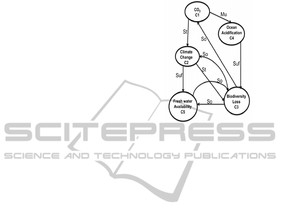
3.1 Feedback
The equilibrium is reached among nodes 2, 3, 4, 5,
and 11 where it exists feedback. They remain ON,
even though the other nodes are OFF. This fact says
that once these nodes are turn on, they remain ON,
and this does not depend on the rest of the system.
If we analyzed the subsystem of nodes 2, 3, 4, 5 and
11 (that represent CO
2
growth, Climate Change, Bio-
diversity Loss, Ocean Acidification, and Fresh Water
Availability, respectively) renamed as 1, 2, 3, 4, and 5
we have:
Figure 3: System of nodes 2, 3, 4, 5, and 11 renamed as 1,
2, 3, 4, and 5 respectivelly.
M
subsystem
=





0 1 0 1 0
0 0 1 0 1
1 1 0 0 1
0 0 1 0 0
0 0 1 0 0





If we force the first node in each step, in two iter-
ations we get a = [1, 1, 1, 1, 1]. And when we ac-
tivate C
1
only in (a
0
) the system also converges to
a = [1, 1, 1, 1, 1] in five steps. This means that when-
ever the node C
1
is activated, at any time, the system
converges into a point, and the feedback remains. To
analyze the system behavior we add fuzzy weights to
the edges. We consider (in this case) four quantifiers
for each edge value some, sufficient, much, strong, and
associate the values in [0, 1] as follows some = 0.25,
sufficient = 0.5, much = 0.75 and strong = 1. These
values correspond to the maximum membership val-
ues for each linguistic set. This is shown in figure 4.
With these values the system matrix is expressed
as:
M
subsystem
=





0 1 0 0.75 0
0 0 1 0 0.5
0.25 0.25 0 0 0.25
0 0 0.5 0 0
0 0 0.25 0 0





Turning ON C
1
and keeping a[1] = 1 after each itera-
tion the system converges to the vector:
a
3
= [1.00, 1.00, 1.00, 0.75, 0.75]
When we turn on the first node only at the first itera-
tion the state vector shows the following behavior:
a
0
= [1, 0, 0, 0, 0]
SIMULTECH2012-2ndInternationalConferenceonSimulationandModelingMethodologies,Technologiesand
Applications
514

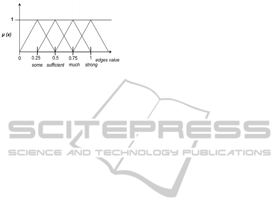
Figure 4: The x-axis represents the values of the causal-
ity between nodes divided in four sets. The y-axis repre-
sents the membership degree of each value in the x-axis for
each fuzzy set. In this manner, 0.25 belongs to the set of
some causality with a membership degree µ(0.25) = 1 rep-
resented in the y-axis. The value 0.75 belongs to the set
sufficient with a membership degree of 1 and so on.
a
1
= [0, 1, 0, 0.75, 0]
a
2
= [0, 0, 1, 0, 0.5]
a
3
= [0.25, 0.25, 0.25, 0, 0.25]
a
4
= [0.03, 0.28, 0.31, 0.18 0.15 ]
a
5
= [0.07, 0.10, 0.41, 0.02 0.21]
a
6
= [0.10, 0.18, 0.17, 0.05 0.15]
a
7
= [0.04, 0.14, 0.25, 0.07 0.13]
.
.
.
a
20
= [0.01, 0.02, 0.04, 0.01 0.02]
Which means that if we force the system only
at t
0
the system tends to the equilibrium vector
a
eq
= [0, 0, 0, 0, 0]. In these case the matrix coef-
ficients represent the system damping to the initial
perturbation. The system behavior given this par-
ticular structure can be interpreted in terms of the
scenarios and mitigation actions, e.g. can the matrix
weights be modified by specific actions or strategies?
3.2 Fuzzy Weighted System
The matrix associated with the fuzzy system is shown
in figure 5.
Turning on the node C
1
we have (a
0
= [1 0 0 0 0
0 0 0 0 0 0 0]), and iterating, the system converges
in two steps into vector: a
∗
2
= [1.00, 1.00, 1.00, 1.00,
0.75, 0.37, 0.87, 1.00, 1.00, 0.75, 1.00, 0.5]
Here we have forced C
1
, i.e. at each iteration a[1] = 1.
We found that the nodes 3, 5, 6, 7, 8, 10, and 12,
reach stable values, while the nodes 2, 4, 9, and 11,
have been limited to 1 by the threshold function.
This offers important information about the network.
As nodes 2, 4, 9, and 11 diverge, they could be
interpreted as sensitive nodes, i.e. these are the nodes
that can not reach an equilibrium with the present
conditions. Then, for example, is possible to think
about short-term actions for them in order to avoid
unwanted scenarios. Furthermore we can say that
even thought the forcing node is industrialization,
mitigation actions may be focused in more than one
node. When we restart C
1
only at t
0
the system is
damping again by the matrix coefficients.
a
1
= [0, 1.00, 0, 0, 0, 0, 0.5, 1.00, 1.00, 0,
0.75, 0.5]
a
2
= [0, 0.37, 1.00, 1.00, 0.75, 0.37, 0.37, 0, 0.75,
0.75, 0.37, 0]
In a
2
the node 4 has been thresholded form 1.18 to 1,
these is because this node has the greatest causality
in the network.
a
3
= [0, 0.53, 0.71, 1.00, 0.28, 0, 0, 0.09, 0, 0, 0.75,
0]
In a
3
the node 4 has been thresholded again.
a
4
= [0, 0.25, 0.78, 1.00, 0.39, 0, 0, 0, 0.07, 0.07,
0.60, 0]
In a
4
we also threshold node 4 from 1.07 to 1
a
5
= [0, 0.25, 0.5, 1, 0.18, 0, 0, 0, 0, 0, 0.64, 0]
In a
5
node 4 is threshold from 1.15 to 1
a
6
= [0, 0.25, 0.5, 0.75, 0.18, 0, 0, 0, 0, 0, 0.5, 0]
In step 6 node 4 need no threshold. From these point
the system converges to zero.
a
7
= [0, 0.18, 0.43, 0.71, 0.18, 0, 0, 0, 0, 0, 0.43, 0]
.
.
.
a
14
= [0, 0.08, 0.17, 0.29, 0.07, 0, 0, 0, 0, 0, 0.18, 0]
We can see how the subsystem with feedback re-
mains, but converges to zero as iterations progress.
The fact that the node 4 diverges give us important
information about the sensibility of this node to the
network conditions, i.e. node 4 has strong sensibility.
Another important analysis is what happens when
the network is at equilibrium and then the conditions
change? In order to analyze this we consider the
vector a
∗
2
that we obtained while maintaining forc-
ing. Then turn off the first node and calculate a∗M
sist
.
a
0
= [1.00, 1.00, 1.00, 1.00, 0.75, 0.37, 0.87,
1.00, 1.00, 0.75, 1.00, 0.5]
a
1
= [0, 1.90, 1.34, 3.18, 0.75, 0.37, 0.87, 1.09, 1.75,
0.75, 1.87, 0.5]
using threshold to limit the values of nodes 2, 3, 4, 8,
9, and 11
a
1
= [0, 1.00, 1.00, 1.00, 0.75, 0.37, 0.87, 1.00, 1.00,
0.75, 1.00, 0.5]
in the second iteration we have:
a
2
= [0, 0.90, 1.00, 1.00, 0.75, 0.37, 0.37, 0.09, 0.75,
0.75, 1.00, 0]
UseofFuzzyCognitiveMapsforClimateSystemStabilityAnalysis
515

Figure 5: Weighted system.
where we also used the treshold function for nodes 3,
4 and 11. At iteration 10 we have:
a
10
= [0, 0.13, 0.29, 0.49, 0.12, 0, 0, 0, 0, 0, 0.34, 0]
Which shows that once forcing is removed,
the system reaches the equilibrium at a
n
=
[0, 0, 0, 0, 0, 0, 0, 0, 0, 0, 0, 0], where the matrix coef-
ficients remain as damping (Liapunov) coefficients.
Nevertheless, it is important to characterize the feed-
back processes in order to know if the threshold func-
tion is changing (or not) the system’s behavior.
3.3 Indirect and Total Effects
(Min-Max)
When we assign fuzzy weights we can use the Indirect
and total effect operators (I and T ) to analyze the
causal action among nodes. Let us analyze, for
example, the causality between industrialization
and biodiversity loss. To go from C
1
to C
4
we
have: (1,2,3,4), (1,7,4), (1,12,11,4), (1,11,4), (1,8,4),
(1,9,4), and (1,12,6,4),(1,12,6,8,4), and (1,12,6,3,4),
which are denoted here as I
1
, I
2
, I
3
, I
4
, I
5
, I
6
, I
7
, I
8
,
I
9
, I
10
respectively. If we analyze the lin-
guistic quantifiers among them: I
1
(C
1
,C
4
) =
min{e
12
, e
23
, e
34
} = min{strong,strong, strong} =
strong. and so: I
2
(C
1
,C
4
) = min{e
17
, e
74
} =
min{su f f icient, strong} = su f f icient.
I
3
(C
1
,C
4
) = min{su f f icient, much, much, su f f icient} =
su f f icient.
I
4
(C
1
,C
4
) = min{su f f icient, much, some} = some.
I
5
(C
1
,C
4
) = min{much, some} = some.
I
6
(C
1
,C
4
) = min{strong, some} = some.
I
7
(C
1
,C
4
) = min{strong, some} = some.
I
8
(C
1
,C
4
) = min{su f f icient, much, su f f icient} =
su f f icient.
I
9
(C
1
,C
4
) = min{su f f icient, much, some, some} =
some.
I
10
(C
1
,C
4
) = min{su f f icient, much, some, strong} =
some.
T (C
1
,C
4
) = max{I
1
, I
2
, I
3
, I
4
, I
5
, I
6
I
7
, I
8
, I
9
, I
10
} =
max{strong, su f f icient, su f f icient, some, some, some,
some, su f f icient, some, some} = strong. Which
means that C
1
“strongly causes” C
4
. The (Min-Max)
analysis give us important information about how
causality is operating in the system, and which
relation or relations among subsystems exert more
influence over one specific node. In the example, we
found that C
1
strongly causes C
4
, however, the only
path that posses strong causality as indirect effect is
I
1
(C
1
,C
4
). We can use this information for strategic
planning, i.e. to modify the action that C
1
exerts
over C
4
(the total effect T), we must focus on the
relations e
12
, e
23
, and e
34
rather than the other edges.
Changing only one of these relations, the total effect
of C
1
over C
4
will change to sufficient.
4 CONCLUSIONS
Throughout this work we build a model for the earth
climate system by relating earth subsystems recog-
nized by experts as those which determine the climate
system stability. In the analysis we found that with
the established network conditions, and considering
only positive causality, the system diverges, which
means that all nodes increase without limit leading
the system into an undesired state. Then, we turn
off the system’s forcer in order to identify the feed-
back processes. Nodes with feedback are specially
important for us as the causality persists among them,
even though the forcing has been turned off. So,
these nodes need special attention because the sys-
tem behavior depends on the edges weight, once a
SIMULTECH2012-2ndInternationalConferenceonSimulationandModelingMethodologies,Technologiesand
Applications
516

node is activated. When we focus on the subsystem
with feedback, we discover that without the forcer the
system returns to the equilibrium state, even without
threshold. Still, we use the threshold function when
working with the complete system. It is necesary
to explore in greater depth the connection edges and
their weights to know if the system is really modeling
these interactions.
The system behavour starting in a particular state
exhibits all the behavours mentioned above, however
the threshold use is stronger in this case, which also
suggests the necesity of refining the weights among
subsystems.
With respect to the Min/Max criteria, we found
that the trayectory (I
1
) with more weight between the
forcer (C
1
) and the node with more entries in the net
(C
4
) is the one that goes from 1 to 2, from 2 to 3 and
from 3 to 4. The analysis of all other possible trayec-
tories shows that the indirect effects of each one are
less than those of I1. To modify the causality of C
1
over C
4
, we have to focus only on the indicated trayec-
tory, i.e. if we change the other trayectories we would
not change the weight over the C
4
node. This is one
of the examples where the cognitive map allow us to
make strategic decisions about a net.
Finally, the use of cognitive maps in climate sys-
tems allows the creation of knowledge networks that
integrate systems that under any other circumstance
would be impossible to integrate to obtain cualitative
information of the system that can be easily adapted
to decision making schemes.
ACKNOWLEDGEMENTS
The present work was developed with the support of
the Programa de Investigaci
´
on en Cambio Clim
´
atico
(PINCC) of the Universidad Nacional Aut
´
onoma de
M
´
exico (UNAM).
REFERENCES
Foley, J. A. (2010). Boundaries for a healthy planet. Scien-
tific American.
Kosko, B. (1986). Fuzzy cognitive maps. Man-Machine
Studies, 24:65–75.
Mace, G., Masundire, H., Baillie, J., Ricketts, T., and
Brooks, T. (2005). Ecosystems and human well-being:
Current state and trends, chapter Chapter 4: Biodiver-
sity. Island Press USA.
on Climate Change, I. I. P. (2007). Cambio clim
´
atico 2007:
Informe de s
´
ıntesis. contribuci
´
on de los grupos de tra-
bajo i, ii y iii al cuarto informe de evaluaci
´
on del
grupo intergubernamental de expertos sobre el cam-
bio clim
´
atico. IPCC, Suiza.
Rockstrm, J., Steffen, W., Noone, K., Persson, Chapin,
F. S., Lambin, E. F., Lenton, T. M., Scheffer, M.,
Folke, C., Schellnhuber, H. J., Nykvist, B., Wit, C. A.,
T., H., Van der Leeuw, S., Rodhe, H., Srlin, H., Sny-
der, P. K., Costanza, R., Svedin, U., Falkenmark, M.,
Karlberg, L., Corell, R. W., Fabry, V. J., Hansen, J.,
Walker, B., Liverman, D., Richardson, K., Crutzen,
P., and Foley, J. A. (2009). A safe operating space for
humanity. Nature, 461.
Stylios, C. D., Georgopoulos, V. C., and Groumpos, P. P.
(1997). The use of fuzzy cognitive maps in modeling
systems. In 5th IEEE Mediterranean Conference on
Control and Systems MED5 paper, volume 67, page 7.
UseofFuzzyCognitiveMapsforClimateSystemStabilityAnalysis
517