Approximation of Geometric Structures with Growing Cell Structures

and Growing Neural Gas

A Performance Comparison

Hendrik Annuth and Christian-A. Bohn

Computer Graphics & Virtual Reality, Wedel University of Applied Sciences, Feldstr. 143, Wedel, Germany

Keywords:

Growing Cell Structures, Growing Neural Gas, Smart Growing Cells, Surface Reconstruction.

Abstract:

We compare Growing Cell Structures and Growing Neural Gas, which were introduced by Bernd Fritzke and

which are famous for their facilities in classiﬁcation, clustering, dimensionality reduction, data visualization,

and approximation tasks. We practically test and analyze their capabilities in geometric approximation and

focusing on the application of surface reconstruction from 3D point-data. Our focus is to work out the differ-

ences of the algorithms that are especially relevant concerning approximation purposes. We address the issue

of suitable input data, their applied graphs, their topological properties, their run time complexities and we

present a summary of suggested alternations to both approaches and evaluate our results.

1 INTRODUCTION

The approximation of a geometric structure M is usu-

ally based on measured data or data received from an

analytically unknown function. The input data is a

point set P = {p

...p

} with a certain dimension n

which also deﬁnes the dimension of the target space

of the approximation. Therefore P = {p

...p

} ⊂

. The dimension n

of the resulting structure

M usually is a subspace of n

. For surface recon-

struction e.g. we have 3D Points P ⊂ R

and our

resulting structure is a 2D surface so n

= 2. With

this deﬁnition given, a geometric approximation re-

constructs a structure M of a certain dimension n

greater zero from a set of points P contained in an n

dimensional target space. With the steady develop-

ment in scanning technologies the amount of data, the

areas of application, and the related challenges con-

stantly rises. The most common problems are noise,

none uniform sample densities, holes in the sample

data, and discontinuities of the tangent space like cor-

ners or creases which cause a huge demand for algo-

rithms that can handle such problems.

2 PREVIOUS WORK

As Geometric approximations demand stability and

robustness due to the presence of noisy data, many

neural computation techniques have been applied to

the problem as well. One of the most important works

in that area of classiﬁcation and clustering is (Mac-

Queen, 1967). In the process k n

-dimensional refer-

ence vectors are placed in the input samples P such

that they are means of those samples. When M is

a graph M = {v

...v

} and C = {c

...c

} ∧ C ⊂

M × M where v is a reference vector and c a connec-

tion between two reference vectors. Kohonen’s self-

organizing-map (SOM) (Kohonen, 1982) and Neural

Gas (Martinetz and Schulten, 1991; Martinetz and

Schulten, 1994) are concepts that introduce M is as a

graph. Since these methods produce topologies, they

successfully can be used for reconstruction purposes.

In (Barhak and Fischer, 2002; Yu, 1999; Hoffmann

and Vrady, 1998) a SOM and in (Melato et al., 2008)

the neural gas approach is used for surface reconstruc-

tion. As the resolution of the reference vectors is

ﬁxed the results strongly depend on the initial posi-

tions of reference vectors and the number of required

reference vectors to properly represent the underlying

geometry needs to be known in advance. Fritzke’s

Growing Cell Structures (GCS) approach (Fritzke,

1993) tracks the approximation error and adds refer-

ence vectors in areas of big approximation error and

terminates when a certain error is reached. Thus the

process does not require a previous choice of resolu-

tion. Growing neural gas (GNG) (Fritzke, 1995) also

tracks the approximation error to add new vectors and

also does not need a predetermined number of refer-

552

Annuth H. and Bohn C..

Approximation of Geometric Structures with Growing Cell Structures and Growing Neural Gas - A Performance Comparison.

DOI: 10.5220/0004157405520557

In Proceedings of the 4th International Joint Conference on Computational Intelligence (NCTA-2012), pages 552-557

ISBN: 978-989-8565-33-4

 2012 SCITEPRESS (Science and Technology Publications, Lda.)

ence vectors. To establish a topology it uses competi-

tive Hebbian learning. Both methods, GCS and GNG,

have been applied to surface reconstruction success-

fully. (Vrady et al., 1999) suggested using GCS

for surface reconstruction the ﬁrst time. Ivrissimtzis

presents modiﬁcations (Ivrissimtzis et al., 2003b) for

mesh smoothing and for adding and deleting refer-

ence vectors with improved connectivity properties.

With the Smart Growing Cells approach (SGC) (An-

nuth and Bohn, 2012) the GCS are enhanced with lo-

cally individual behavior to, ﬁrst, account for surface

curvature through the granularity of the underlying

topology of the graph. Second, complex homeomor-

phisms can be reconstructed, and third, tangential dis-

continuities like corners and creases are reconstructed

correctly. In (Holdstein and Fischer, 2008; Do R

ego

et al., 2010; Melato et al., 2008) GNG was used for

surface reconstruction while in (do Rego et al., 2007)

a hybrid approach using both, GCS and GNG, for sur-

face reconstruction is presented.

3 PERFORMANCE

COMPARISON

In this section we analyze similarities and differences

of both approaches, and compare their strengths and

weaknesses in the area of geometric approximation.

We use surface reconstruction in our examples since

it is a very common type of application of these algo-

rithms.

3.1 Similarities of GCS and GNG

GCS and GNG both introduce a stochastic approach

to the problem of geometric approximation. The sam-

ple points in P are accessed in a random series. This

gives the method a big advantage. At any given time

during the iterations only one data sample of P needs

to be loaded. Therefore such approaches can process

as many measured points as a modern hard drive is

able to contain. Since both algorithms are descents

from classical k-means clustering, they are both very

strong against noisy data (see Fig. 1). Their algo-

rithms are fairly simple and easy to understand. This

makes these algorithms maintainable and as both con-

cepts are actually based on data analysis they can

robustly cope with any given point constellation P .

GCS and GNG are also very ﬂexible. While P is pro-

cessed, points could be added or deleted from P , or

regions of special interest in P could be set to a higher

likelihood within the random sample selection, which

would create a higher resolution in those areas (Hold-

stein and Fischer, 2008). The processes can also be

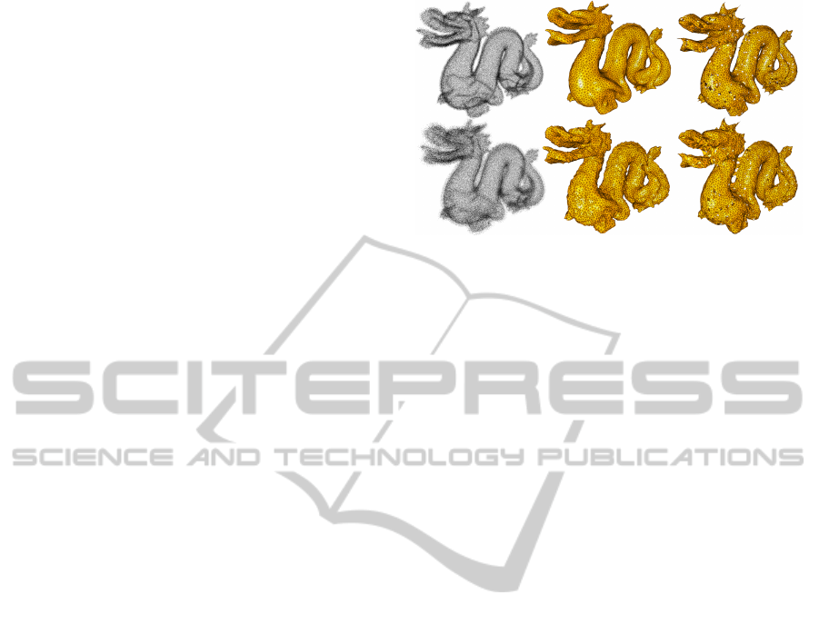
Figure 1: Both algorithms have a natural ability to deal with

noise data. Point Cloud (left), GCS (middle), GNG (right),

2% Gaussian noise (top) and 4% Gaussian noise (bottom).

stopped or continued at any given time during the iter-

ations. On the downside both create M as a mesh and

not as differentiable smooth approximation. Fritzke

presented a GNG concept that uses radial basis func-

tions (Fritzke, 1996), but this concept has not jet been

used for geometric approximation purposes.

3.2 Sample Points P

The approximation of a geometric structures from P

basically exposes two kinds of problems. First, not

all points in P might interpolate M due to noise or

outliers. As mentioned above section 3.1 this kind of

problems can be satisfactory handled by both algo-

rithms. Second, the amount of points that is needed

for an algorithm to create a sound surface — here

GCS and GNG differ. The basis of existence for a

structure in M and its associated topology C is carried

at different places in the algorithms. In GCS the sig-

nal counters of a reference vector determines whether

a reference vectors is deleted or not. In GNG the dele-

tion is determined by the age of the connections be-

tween reference vectors. In order for both structures

to remain they need to be hit by a sample point. As

|M | is way smaller then |C|, a GNG Graph simply

needs more points to create a equivalent approxima-

tion (see Fig. 2). In an ideal situation for M every

reference vectors has six connections. This is ideal,

because every triangle can potentially be an equilat-

eral triangle in such a constellation and the reference

vectors are as evenly distributed as possible, which is

desirable for most processes in computer graphics.

If every connection in C has two triangles on both

sides, which means the surface has no boundaries, we

can calculate the required points for both algorithms

in an ideal case. For GCS any signal counter is associ-

ated with one reference vector, in order to get a signal

at some time, |M | should not exceed the amount of

points |P |. For GNG in an ideal scenario were any

ApproximationofGeometricStructureswithGrowingCellStructuresandGrowingNeuralGas-APerformance

Comparison

553

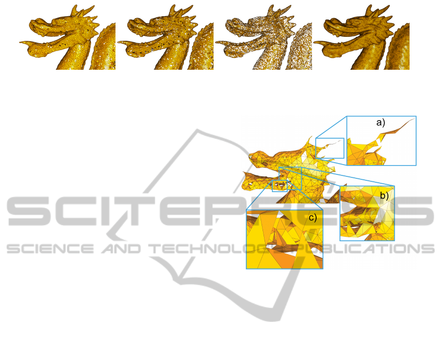
Figure 2: When the number of points in the GNG process in not sufﬁcient to hit the connection in the graph, the structure

starts to dissolve. From left to right approximations with different numbers of reference vectors: GNG Dragon 30K, GNG

Dragon 60K, GNG Dragon 120K and GCS Dragon 120K.

vertex has six connections, which are shared by two

reference vectors |C | = 3 · |M |, so |M | can only be

a third of |P | in an ideal scenario. In (Holdstein and

Fischer, 2008) and in our tests we discovered by prac-

tical testing that the best results are created at 5% to

10% of |P |.

3.3 Graph M

For GCS and GNG M is a speciﬁc graph. GCS is

only allowed to include simplices of the previous cho-

sen dimension n

, while M in the case of GNG can

contain any kind of simplex that does not exceed the

dimension n

. If n

is unknown or even needs to be

a set of values, GCS is simply impractical, but in case

of geometric approximation this is seldom if ever the

case. The problem is usually the other way round. So

is known, in case e.g. of surface reconstruction

it is 2D, but in GNG M is not guaranteed to con-

sist of triangles. Therefore a post process needs to

delete or transform all structures in M with a differ-

ent dimension then 2D and those which infringe the

criteria for a manifold. Which means that a connec-

tion c ∈ C can be connected to a maximum of two

triangles. Since the process naturally creates lots of

polygons with more then three sides, the process also

needs to include a hole ﬁlling mechanism (see Fig.

3).

In our implementation we did not introduce such a

method to give an impression of the result of the ac-

tual GNG algorithm, as such a method could be im-

plemented in many different ways leading to very dif-

ferent results for M . For our Figures we will show M

as a graph of triangles, that do not have an orientation.

Neither GCS nor GNG deﬁne an oriented surface in

M . In a real world computer graphics application

however, a graph M needs to have oriented triangles.

Even so this is not part of the actual GCS deﬁnition,

all reconstruction algorithms we encountered in our

research used a graph that already includes oriented

triangles. As the surface is reﬁned within the process,

it is always build based on pre-existing surface. This

way the orientation and gradient of a surface has a cer-

tain inertia, which enables the process to create sound

Figure 3: Different possible constellations in a GNG graph,

like a none-manifold connection that is attached to three tri-

angles a), many holes in the surface b) and connection that

rather present a volume than a surface c).

surfaces even in very challenging areas of P . If the

surface is incorrect however this inertia might prevent

surface from being corrected and an initial orienta-

tion, does not generally prevent the GCS process from

creating twisted surface (see section 3.4).

Since M is not necessarily exclusively build of trian-

gles in the GNG approach, M cannot be implemented

as a graph consisting of oriented triangles through-

out the process. Therefore reﬁnements in M are not

based on pre-existing surface. The topology gener-

ating method in the GNG process is not guided by

previous surface stages. When the process is ﬁnished

and the necessary cleaning mechanism has been per-

formed on M the orientation of the encountered tri-

angles need to be propagated across the graph, which

can especially in noisy areas lead to twisted surface

(see (Holdstein and Fischer, 2008)). As GCS uses

a more sophisticated graph, a lot more information

can be deduced within the process, depending the sur-

face gradient or triangle properties like normal vec-

tors. This extra information can be used to augment

the algorithm (see section 3.6).

3.4 Topology C

In the following section we will focus on the algo-

IJCCI2012-InternationalJointConferenceonComputationalIntelligence

554

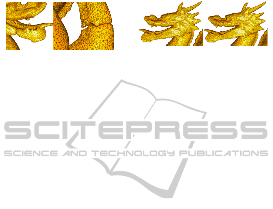
Figure 4: At the mouth of the Dragon the GCS process

ran in a local minimum (left). The tail of the Dragon can

not be approximated correctly, since the process was ini-

tialized with a tetrahedral, which has a different genus than

the Dragon(right).

rithms topologies. In case of GNG every topology can

be constructed, which is more a problem in the subse-

quent cleaning process. So without any modiﬁcation

GNG can actually produce any demanded topology.

In case of GCS that is not the case. The surface can

only create topologies equal to the initial topology.

New added reference vectors always preserve the pre-

existing surface (this can also be an advantage section

3.3). This creates two problems, ﬁrst the surface can

tangle up in a local minimum and second if P is based

on a structure of different topology, it cannot be cor-

rectly build (see Fig. 4). To choose the demanded

topology in advance, would not solve the problem,

since the process would still run into local minima

and for any approximation the topology would need

to be known in advance. The standard GCS algo-

rithm is practically unable to create approximations

for topologies of different genus. This problem how-

ever has successfully been dealt with (see section 3.6).

3.5 Run Time Complexity

Without any aide of supporting algorithms the run

time complex of both GCS and GNG is O(n

), where

n dependents on the ﬁnial approximation resolution

|M |. The basic step that is performed depended on

the approximation resolution |M | includes the search

for the nearest neighbor in M to a given sample point,

which naively implemented includes a distance check

to all reference vectors in M (O(n)). This search can

be improved by using an Octree, which reduces the

complexity of this search to O(logn). The basic step

also contains decreasing the collected error of all ref-

erence vectors O(n). And the adding and deletion

process includes to ﬁnd the highest or lowest error

under all reference vectors O(n). This has been ad-

dressed in (Annuth and Bohn, 2010b), where a data

structure called Tumble-Tree reduces these complex-

ities to O(logn). So the overall run time complexity

of both algorithms can be reduced to O(nlogn).

Figure 5: The GCS process with the smoothing operation

(left) shows triangles that are closer to equilateral triangles,

than the standard neighbor moving technique (right).

3.6 Modiﬁcation Overview

In the following sections, we want to present some

modiﬁcations that have been suggested to enhance

both approaches.

GCS: For approximations of a certain size a con-

stant error counter decreasing degree β is impractical,

because all error counters start to converge to zero.

Therefore (Ivrissimtzis et al., 2003a) introduce a dy-

namic β value. β = 1 − η

1/((γ=6)·|M |)

γ is the number of times a reference vector is allowed

to be missed, before it falls under the deletion thresh-

old η. In (Ivrissimtzis et al., 2003b) the moving of

neighbors was exchanged for a smoothing mechanism

presented by Taubin (Taubin, 1995). This increased

the overall triangle quality, measured in equilateral

triangles (see Fig. 5). In (Ivrissimtzis et al., 2003b)

the way how new reference vectors are added and

deleted is improved. The presented processes mostly

create reference vectors with six connections which

again creates more equilateral triangles. The GCS ap-

proximation creates a surface of simplices. In areas

of curved surface a higher resolution of triangles is

needed then in plane areas to reach the same approx-

imation quality. This has been issued in (Jeong et al.,

2003) where the change in normal directions has been

tracked and to add more reference vectors in such area

of much movement. In (Annuth and Bohn, 2010a) the

global curvature is set in relation to the local curvature

of a reference vector. If the local curvature is higher

signals in such an area count more, which leads to

more reference vectors in those areas. (Annuth and

Bohn, 2012) presents a general concept of enhancing

the GCS approach, the Smart Growing Cells (SGC).

The concept introduces individual behavior for the

reference vectors. That means that for different sit-

uations in the graph, the adaption process alters. The

biggest challenge is the inability of GCS to model

Surface of different genus (see Fig. 4). The presented

process in (Ivrissimtzis et al., 2003b) had no mecha-

nism to cut or coalesce the surface. In (Ivrissimtzis

et al., 2003a) the cutting of surface was triggered by

the size of triangles and then coalescing by a certain

threshold for the Hausdorff distance of two bound-

ApproximationofGeometricStructureswithGrowingCellStructuresandGrowingNeuralGas-APerformance

Comparison

555

aries. This method has two important disadvantages.

First the triangle sizes that reliably indicates misplace

surface takes quite a long time to appear and second

in case of none uniform sample densities where tri-

angle naturally have different sizes the system does

not work. Excluding those sample distributions again

would destroy a big advantage of the whole approach.

In (Annuth and Bohn, 2010a) the cutting is triggered

by a high number of connections |N

| of a reference

vector v. This mechanism detects misplaced surface

a lot faster and also works for none uniform sample

densities. The coalescing process happens dynami-

cally when equally oriented boundaries come close to

each other.

GNG. Both methods (Do R

ego et al., 2010; Melato

et al., 2008) introduced an operation which changes

the amount of iterations λ before adding reference

Vectors. In (Melato et al., 2008) with increasing size

|M | they increase the size of λ. In (Do R

ego et al.,

2010) after the demanded size |M | was reached they

introduced another learning phase, where only topol-

ogy is learned, but no additional reference vectors

were added. The reason for this operations is that the

basic reference vector adding step creates holes, be-

cause it creates reference vectors that have two con-

nections. A different approach to tackle this problem

is presented in (do Rego et al., 2007), were they mod-

iﬁed the basic adaption step and the adding step. They

search for three instead of two closest points to a ran-

dom sample p. By that they tried to insure that the

process creates triangles rather than arbitrary dimen-

sional structures. The adding of reference vectors was

done according to the GCS method, for this M had

to be an triangle based graph. The problem with this

concept is that the connections that are made in the ba-

sic step are still arbitrary, therefore the approach still

creates cross connections and overlapping triangles.

4 RESULT

In this paper we practically compared the perfor-

mance of GCS and GNG and worked out differences

and explained their meaning towards the approxima-

tion process. In the following we show results with

different parameter modiﬁcations. To make them

comparable we used the Stanford Dragon with a ﬁxed

resolution |M | of thirty-thousand reference vectors.

The model has uneven point densities, some detail ar-

eas like the horns and a relatively challenging from.

We measure point distance, valence, triangle quality

and the run time. The following results have been

calculated single threaded on a 2.53GHz CPU.

We measure the distance after root-mean-square

Table 1: The table shows our results for the Stanford

Dragon build of 30K reference vectors, under different cir-

cumstances.

RMS ·10

val Tri Qual time

Benchmark

GCS 3.83 0.900 0.785 17.3sec

GNG 8.31 0.679 0.636 6.6sec

Neighbor Move vs Smooth

GCS 5.48 0.861 0.610 13.3sec

Different # of smoothing rounds

GCS 5 4.10 0.905 0.786 40.3sec

GCS 20 4.08 0.907 0.790 234.4sec

Different λ

GNG 200 8.11 0.802 0.675 12.3sec

GCS 200 3.72 0.906 0.787 35.3sec

GNG 400 8.13 0.873 0.705 24.8sec

GCS 400 3.59 0.913 0.789 75.8sec

GNG 2000 7.84 0.944 0.750 113.4sec

GCS 2000 3.45 0.924 0.790 415.2sec

Different a

max

GNG 44 7.97 0.797 0.685 6.5sec

GNG 176 12.38 0.318 0.459 6.4sec

(RMS). As the surface of GNG is not sealed, only

points directly above or beneath triangle are included.

We deﬁne the distance one as the diagonal of the

bounding box of P . The valence of a reference vector

v is its number of it’s connections |N

|, we measure

the degree of reference vectors that have a valence

from ﬁve to seven. We measure the triangle quality

as the average closeness of a triangle to an equilateral

triangle. We calculate the surface area A of an trian-

gle t. Then we calculate the surface area A

of second

triangle t

. t

is an equilateral triangle with the side

length of the longest side of t. Then we divide A by

. In our benchmark versions we used the param-

eters as presented in (Annuth and Bohn, 2010a) and

for GNG as in (Fritzke, 1995).

In our test we investigate for GCS the neighbor

smoothing process and different values for λ. For

GNG we will use different values for λ and different

maximum lifespans for the edges a

max

(see table 1).

5 CONCLUSIONS

Both algorithms have great potential in geometric ap-

proximation, because of their resistance to noise and

none uniform sample densities and because of their

independence of sample set sizes. For structures of

mixed or unknown dimension GNG is capable of an

approximation, even so we could not think of a prac-

tical use case. Apart from that the algorithm needs in-

IJCCI2012-InternationalJointConferenceonComputationalIntelligence

556

herently more points to reconstructed an approxima-

tion of the same resolution in comparison to the GCS

approach. Thru low age

max

values triangles quality

can be gained in exchange for more holes in the sur-

face. Thru λ time can be exchanged for an overall

better approximation. We found the best trade of at

age

max

= 88 and λ = 200. GNG needs a cleaning

phase, that can only be done in a post-process. How-

ever we think that an GNG approach based on radial

base functions might has the potential to overcame

some of these disadvantages.

The GCS approach is less time efﬁcient, which is

mostly due to its more sophisticated graph. The

smoothing operation, is also time consuming, but has

very positive effects on the valance, triangle quality

and also the distance to the points. Note that this op-

eration cannot be used for GNG, since the operation

uses triangle normals.

In our analysis of these approaches we came to the

conclusion that the progressively evolving surface in

the GCS approach and the ability to augment the pro-

cess with enhancing operations that smoothly inte-

grate in the process due to the more sophisticated base

graph makes the process is in context of geometric ap-

proximation overall to the superior technique.

REFERENCES

Annuth, H. and Bohn, C.-A. (2010a). Surface reconstruc-

tion with smart growing cells. Studies in Computa-

tional Intelligence, 321:47–66.

Annuth, H. and Bohn, C. A. (2010b). Tumble tree: reduc-

ing complexity of the growing cells approach. In Pro-

ceedings of the 20th international conference on Ar-

tiﬁcial neural networks: Part III, ICANN’10, pages

228–236, Berlin, Heidelberg. Springer-Verlag.

Annuth, H. and Bohn, C.-A. (2012). Smart growing cells:

Supervising unsupervised learning. In Madani, K.,

Dourado Correia, A., Rosa, A., and Filipe, J., editors,

Computational Intelligence, volume 399 of Studies in

Computational Intelligence, pages 405–420. Springer

Berlin / Heidelberg. 10.1007/978-3-642-27534-0 27.

Barhak, J. and Fischer, A. (2002). Adaptive reconstruction

of freeform objects with 3d som neural network grids.

Computers & Graphics, 26(5):745–751.

do Rego, R. L. M., Arajo, A. F. R., and de Lima Neto,

F. B. (2007). Growing self-organizing maps for sur-

face reconstruction from unstructured point clouds. In

IJCNN, pages 1900–1905. IEEE.

Do R

ego, R. L. M. E., Ara

ujo, A. F. R., and De Lima Neto,

F. B. (2010). Growing self-reconstruction maps.

Trans. Neur. Netw., 21(2):211–223.

Fritzke, B. (1993). Growing cell structures - a self-

organizing network for unsupervised and supervised

learning. Neural Networks, 7:1441–1460.

Fritzke, B. (1995). A growing neural gas network learns

topologies. In Tesauro, G., Touretzky, D. S., and Leen,

T. K., editors, Advances in Neural Information Pro-

cessing Systems 7, pages 625–632. MIT Press, Cam-

bridge MA.

Fritzke, B. (1996). Automatic construction of radial basis

function networks with the growing neural gas model

and its relevance for fuzzy logic. In Proceedings of the

1996 ACM symposium on Applied Computing, SAC

’96, pages 624–627, New York, NY, USA. ACM.

Hoffmann, M. and Vrady, L. (1998). Free-form surfaces for

scattered data by neural networks. Journal for Geom-

etry and Graphics, 2:1–6.

Holdstein, Y. and Fischer, A. (2008). Three-dimensional

surface reconstruction using meshing growing neural

gas (mgng). Vis. Comput., 24:295–302.

Ivrissimtzis, I., Jeong, W.-K., and Seidel, H.-P. (2003a).

Neural meshes: Statistical learning methods in surface

reconstruction. Technical Report MPI-I-2003-4-007,

Max-Planck-Institut f”ur Informatik, Saarbr

ucken.

Ivrissimtzis, I. P., Jeong, W.-K., and Seidel, H.-P. (2003b).

Using growing cell structures for surface reconstruc-

tion. In SMI ’03: Proceedings of the Shape Modeling

International 2003, page 78, Washington, DC, USA.

IEEE Computer Society.

Jeong, W.-K., Ivrissimtzis, I., and Seidel, H.-P. (2003).

Neural meshes: Statistical learning based on normals.

Computer Graphics and Applications, Paciﬁc Confer-

ence on, 0:404.

Kohonen, T. (1982). Self-Organized Formation of Topolog-

ically Correct Feature Maps. Biological Cybernetics,

43:59–69.

MacQueen, J. B. (1967). Some methods for classiﬁcation

and analysis of multivariate observations. pages 281 –

297.

Martinetz, T. and Schulten, K. (1991). A

”Neural-Gas

” Net-

work Learns Topologies. Artiﬁcial Neural Networks,

I:397–402.

Martinetz, T. and Schulten, K. (1994). Topology represent-

ing networks. Neural Networks, 7(3):507–522.

Melato, M., Hammer, B., and Hormann, K. (2008). Neural

gas for surface reconstruction. IfI Technical Report

Series.

Taubin, G. (1995). A signal processing approach to fair

surface design. In SIGGRAPH ’95: Proceedings

of the 22nd annual conference on Computer graph-

ics and interactive techniques, pages 351–358, New

York, NY, USA. ACM.

Vrady, L., Hoffmann, M., and Kovcs, E. (1999). Im-

proved free-form modelling of scattered data by dy-

namic neural networks. Journal for Geometry and

Graphics, 3:177–183.

Yu, Y. (1999). Surface reconstruction from unorganized

points using self-organizing neural networks. In

In IEEE Visualization 99, Conference Proceedings,

pages 61–64.

ApproximationofGeometricStructureswithGrowingCellStructuresandGrowingNeuralGas-APerformance

Comparison

557