Combined Input Training and Radial Basis Function Neural Networks

based Nonlinear Principal Components Analysis Model

Applied for Process Monitoring

Messaoud Bouakkaz and Mohamed-Faouzi Harkat

University Badji Mokhtar-Annaba, P. O. Box 12, Annaba 23000, Algeria

Keywords:

Nonlinear PCA, IT-net, RBF-neural Network, Process Monitoring, Fault Detection and Isolation.

Abstract:

In this paper a novel Nonlinear Principal Component Analysis (NLPCA) is proposed. Generally, a NLPCA

model is performed by using two sub-models, mapping and demapping. The proposed NLPCA model consists

of two cascade three-layer neural networks for mapping and demapping, respectively. The mapping model is

identiﬁed by using a Radial Basis Function (RBF) neural networks and the demapping is performed by using

an Input Training neural networks (IT-Net). The nonlinear principal components, which represents the desired

output of the ﬁrst network, are obtained by the IT-NET. The proposed approach is illustrated by a simulation

example and then applied for fault detection and isolation of the TECP process.

1 INTRODUCTION

Principal component analysis (PCA) is among the

most popular methods for extracting information

from data, which has been applied in a wide range

of disciplines. In process monitoring with Principal

component analysis, PCA is used to model normal

process behavior and faults are then detected by ref-

erencing the measured process behavior against this

model.

It is known that the multivariate projection tech-

nique of PCA is linear, therefore it is only applica-

ble for extracting information from linearly correlated

process data. However, many industrial processes ex-

hibit nonlinear behavior. For such nonlinear systems,

linear PCA is inappropriate to describe the nonlinear-

ity within the process and it can produce excessive

number of false alarms or alternatively, missed detec-

tion of process faults, which signiﬁcantly compromise

the reliability of the monitoring systems.

To cope with this problem, extended versions of

PCA have been developed such as Nonlinear PCA

(NLPCA). Whilst linear PCA identiﬁes the linear cor-

relations between process variables, the objective of

nonlinear PCA is to extract both linear and nonlinear

relationships. Hastie and Stuetzle (Hastie and Stuet-

zle, 1989), proposed a principal curve methodology

to provide a nonlinear summary of a m-dimensional

data set. However, this approach is non-parametric

and can not be used for continuous mapping of new

data. To overcome the parametrization problem, sev-

eral nonlinear PCA based on neural networks have

been proposed (Kramer, 1991), (Dong and McAvoy,

1996), (Tan and Mavrovouniotis, 1995).

Tan and Mavrovouniotis (Tan and Mavrovounio-

tis, 1995) formulated an alternative scheme of non-

linear PCA based on an input-training neural network

(IT-Net). Under this approach, only the demapping

section of the NLPCA model is considered.

Compared with the other neural networks, when

it is in training, its inputs which represent the desired

principal component are not ﬁxed but adjusted simul-

taneously with the internal network parameters, and

it can perform all functions of a ﬁve layer neural net-

work. However, IT-Net has its own limitation. For

example, for a new data set or observation, calcula-

tion of its corresponding nonlinear principal compo-

nent require more computation due to the necessity of

an on-line nonlinear optimizer.

To improve this approach, a NLPCA model com-

binin a principal curve algorithm (Hastie and Stuetzle,

1989) and two cascade three-layer neural networks is

proposed to identify mapping and demapping models

(Dong and McAvoy, 1996).

Harkat et al. (Harkat et al., 2003) proposes a

similar approach which uses two RBF networks for

nonlinear principal component mapping and demap-

ping, respectively. First, the principal curve algo-

483

Bouakkaz M. and Harkat M..

Combined Input Training and Radial Basis Function Neural Networks based Nonlinear Principal Components Analysis Model Applied for Process

Monitoring.

DOI: 10.5220/0004152304830492

In Proceedings of the 4th International Joint Conference on Computational Intelligence (NCTA-2012), pages 483-492

ISBN: 978-989-8565-33-4

 2012 SCITEPRESS (Science and Technology Publications, Lda.)

rithm is used to estimate the principal components.

Then supervised learning is used to train the two RBF

networks. The methodology proposed in this paper

avoids the use of the principal curve algorithm by re-

placing the RBF demapping network with an IT-Net,

which is able to estimate the principal components

during learning.

The NLPCA approach proposed in this study uses

SPE index for fault detection. In the linear version of

PCA, the reconstruction approach, which tries to re-

construct the i

variable from all other variables, is

used for fault isolation (Dunia et al., 1996). Based

on the same idea, we develop a nonlinear version

of reconstruction approach using NLPCA model for

fault isolation and reconstruction of the faulty mea-

surements as in the linear case (Harkat et al., 2003),

(HAR, ).

The outline of this paper is as follows. Sec-

tion 2 presents a Principal Component Analysis ap-

proach. Section 3 gives brieﬂy reviews of some ex-

isting NLPCA methods. Section 4 describes the pro-

posed NLPCA model combining the IT-Net and RBF

neural networks. Section 5 describes the detection

and isolation approach. Section 6 give an illustration

example while section 7 gives the results of applica-

tion of the proposed approach to the Tennessee East-

man process, and ﬁnally conclusions are presented in

the last section.

2 PRINCIPAL COMPONENT

ANALYSIS (PCA)

Principal component analysis (PCA) is a dimension

reduction technique used in multivariate statistical

analysis which deals with data that consist of mea-

surements. The number of variables in such cases is

often impracticably large, and one way to reducing it

is to take linear combinations of variables and discard

those with small variances. PCA looks for a few lin-

ear combinations which can be used to summarize the

data while losing as little information as possible.

Let X represents a N × m matrix of data. PCA is

an optimal factorization of X into matrix T (princi-

pal components N × ℓ) and P (loadings m × ℓ) plus a

matrix of residuals E (N × m).

X = TP

+ E (1)

where ℓ is the number of factors (ℓ < m). The Eu-

clidean norm of the residual matrix E must be min-

imized for a given number of factors. This criterion

is satisﬁed when the columns of P are eigenvectors

corresponding to the ℓ largest eigenvalues of the co-

variance matrix of X. PCA can be viewed as a linear

mapping from ℜ

to a lower dimensional space ℜ

ℓ

The mapping has the form

t = P

x (2)

where x

represents a single row of X and t

rep-

resents the corresponding row of T. The loadings P

are the coefﬁcients for the linear transformation. The

projection can be reversed back to ℜ

with

x = Pt (3)

where

x is the estimated vector of data.

Nonlinear PCA is an extension of linear PCA. Whilst

PCA identiﬁes linear relationships between process

variables, the objective of nonlinear PCA is to extract

both linear and nonlinear relationships. This general-

ization is achieved by projecting the process variables

down onto curves or surfaces (Fig.2) instead of lines

or planes (Fig.1).

In both cases the objective function to be mini-

mized is the sum of squared orthogonal deviations:

min

∑

i=1

−

= min

∑

i=1

− F (G (x

))k

(4)

where x

is the ith row of X, G is the mapping func-

tion and F represents the demapping function. In this

case, the nonlinear mapping has the form

t = G (x) (5)

and the inverse transformation is implemented by the

second nonlinear vector function F that has the form

x = F (t) (6)

Given an N × m matrix representing N measurements

made on m variables, reduction of data dimensional-

ity aims to map the original data matrix to a much

smaller matrix of dimension N × ℓ (ℓ < m), which is

able to reproduce the original matrix with minimum

distortion through a demapping projection. The re-

duced matrix describes principal component variables

extracted from the original matrix (Fig.3).

Figure 1: The linear principal component minimizes the

sum of squared orthogonal deviations using a straight line.

We provide in the next a brief overview of neu-

ral network based NLPCA proposed over the last two

decades and its implementation.

IJCCI2012-InternationalJointConferenceonComputationalIntelligence

484

Figure 2: The nonlinear principal component minimizes the

sum of squared orthogonal deviations using a smooth curve.

X ∈ ℜ

N×m

ℓ

X ∈ ℜ

N×m

Mapping function

T ∈ ℜ

N×ℓ

ℓm

Demapping funtion

Figure 3: Reduction of data dimentionality.

3 NONLINEAR PCA

The objective, is to extract the nonlinear information

from the nominal data set, namely, how to ﬁnd ma-

trix of nonlinear principal component scores T and a

suitable nonlinear function F (t) to satisfy the equa-

tion (4). In this ﬁeld, many neuronal NLPCA ap-

proaches have been developed, (Hastie and Stuet-

zle, 1989), (Kramer, 1991), (Tan and Mavrovounio-

tis, 1995), (Dong and McAvoy, 1996), (Harkat et al.,

2003).

3.1 Five-layer Neural Network based

NLPCA

To perform NLPCA, the Neural Network in Fig.4

contains three hidden layers of neurons between the

input and output layers of variables (Kramer, 1991).

(k)

ˆx

(k)

ˆx

(k)

ˆx

(k)

(x)

(t)

(x)

(t)

(x)

(t)

(k)

Figure 4: Five-layer NLPCA neural network for extraction

one nonlinear principal component.

A transfer function G

maps from x, the input col-

umn vector of length m, to the ﬁrst hidden layer, rep-

resented by h

(x)

, a column vector of length r, with

elements

(x)

= G

∑

i=1

(x)

+ b

(x)

(7)

The mapping function G is deﬁned as

t = G (x) =

∑

j=1

(x)

(8)

Next, a transfer function F

maps from t to the

ﬁnal hidden layer h

(t)

, a column vector of length r,

with elements

(t)

= F



(t)

t + b

(t)



(9)

and the demapping function F is given by

ˆx = F (t) =

∑

j=1

(t)

(x)

(10)

where ˆx representing the estimation vector of the orig-

inal data x The transfer functions G

and F

are gen-

erally nonlinear. The MSE (mean square error) be-

tween the neural network output ˆx and the original

data x is minimized by ﬁnding the optimal values of

(x)

, w

(x)

, w

(t)

, b

(t)

, V

(t)

and

(t)

3.2 Three-layer Neural Network

NLPCA

Dong and McAvoy (Dong and McAvoy, 1996) pre-

sented an NLPCA method which integrates the prin-

cipal curve algorithm and neural networks. The basic

idea is to reduce the ﬁve-layer auto-associative net-

work to a three-layer networks. In a such approach,

two three-layer neural networks have been used. The

inputs of the ﬁrst neural network are the original data,

and the outputs are the nonlinear principal scores ob-

tained by principal curves. The inputs of the second

network inputs are the ℓ nonlinear principal scores ob-

tained by principal curves, and the outputs are the cor-

rected data. Each neural network can be trained sepa-

rately by any appropriate algorithm.

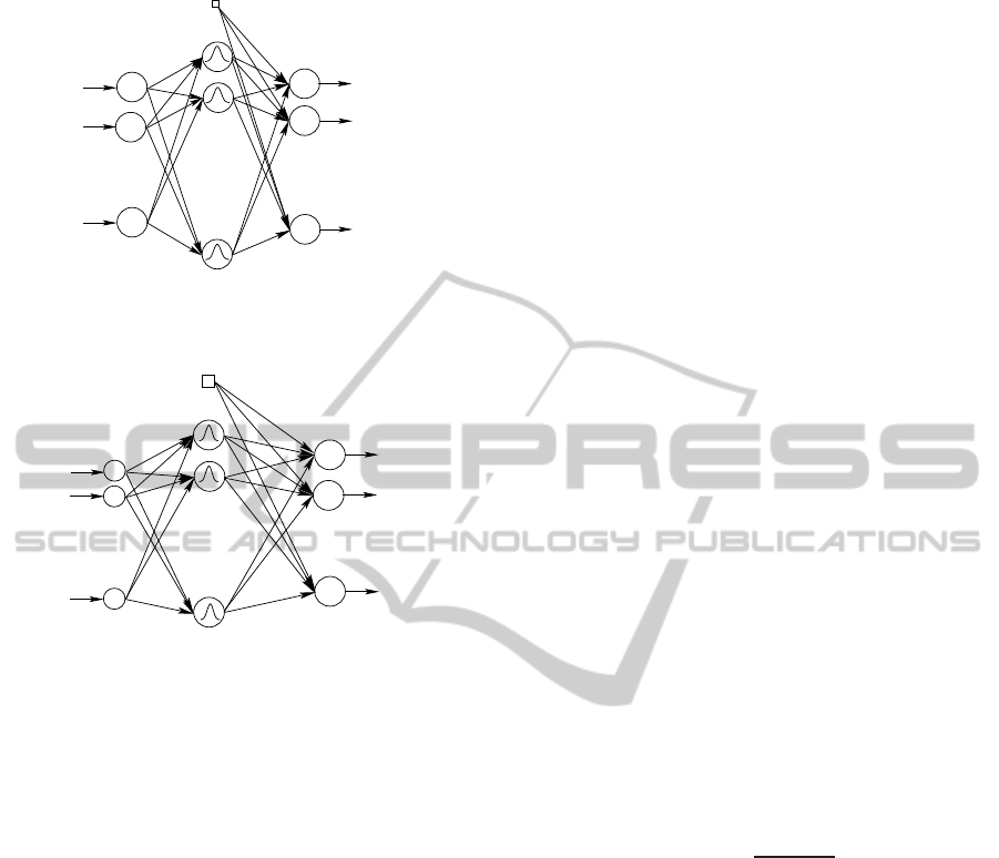
3.3 RBF-NLPCA Model

The nonlinear principal component analysis model

for mapping and demapping can be obtained by us-

ing two RBF-Networks (Fig.5) and (Fig.6).

To identify the RBF-NLPCA model, we determi-

nate the parameters of radial basis functions (centers

and dispersions) and the weight parameters for the

two RBF-networks. It should be noted that the nonlin-

ear principal component matrix T being unknown, the

CombinedInputTrainingandRadialBasisFunctionNeuralNetworksbasedNonlinearPrincipalComponentsAnalysis

ModelAppliedforProcessMonitoring

485

ℓ

Figure 5: RBF-Network for mapping from ℜ

→ ℜ

ℓ

ˆx

ℓ

Figure 6: RBF-Network for mapping from ℜ

ℓ

→ ℜ

training of the two RBF-networks separately is then

impossible.

To overcoming this problem, two solutions have

been proposed for estimating nonlinear principal

component (Webb et al., 1999), (Harkat et al., 2003).

The difference between the two methods is how to

calculate the nonlinear principal component neces-

sary for training of the two RBF neural networks. In

the ﬁrst solution, proposed by Webb (Webb et al.,

1999), use the maximizing of the variance (Webb

et al., 1999), and the second is the combining the

RBF-networks and principal curves.

1. Webb (Webb et al., 1999) proposed an approach to

nonlinear principal component analysis using ra-

dial basis function (RBF) networks. The ﬁrst net-

work projects data onto a lower dimension space

Fig.5, such that the nonlinear features are captured

in the sense of variance maximization of its out-

puts. So, Network parameters are determined by

the solution of a generalized symmetric eigenvec-

tor equation by maximizing the variance of its out-

puts and then nonlinear principal components are

the outputs given by this identiﬁed network.

By preserving the original dimension of the data,

the second network try to perform the inverse

transformation Fig.6 (reproducing the original

data) by minimizing the squared prediction error

between the original data samples and its corre-

sponding outputs. The two networks are trained

separately and the outputs of the ﬁrst one are the

inputs of the second.

However, the optimization task of the ﬁrst net-

work become so difﬁcult because for this opti-

mization we need to minimize estimation error

which lead to train the second RBF-network and

compare its outputs to the inputs of the ﬁrst one.

2. The nonlinear component matrix T is estimated

by using the principal curve algorithm (Hastie

and Stuetzle, 1989), (Verbeek, 2001). Then, each

RBF-network can be trained separately. So, the

training problem is transformed into two classical

nonlinear regression problems. We consider the

RBF neural network illustrated in Fig.5. The aim

is to use this network to deﬁne the nonlinear func-

tion G (.) : ℜ

→ ℜ

ℓ

of x ∈ ℜ

. The outputs are

computed as a linear weighted sum of the hidden

node outputs:

= G (x) =

∑

i=1

(x) (11)

Where t is the output vector of ℓ outputs,

, i = 1, ···i, ··· r) are the output layer weight

parameters matrix W elements to be deter-

mined, connecting hidden node i to output j,

and (

, i = 1, ···i, ··· r) is the gaussian function

given by:

(x) =



kx− c



(12)

Where c

and

respectively denote centers and

dispersions, In this paper, the centers, c

are ob-

tained with C Fuzzy-means clustering method and

the dispersions

are determined as the dis-

tance between c

and the closest c

(i 6= j, j =

{1, ··· ,r}). So the training of the ﬁrst network

needs only to update the parameter weights. The

parameter weights are obtained by a least square

solution minimizing according to deﬁnition (13).

w = (

)

−1

T (13)

Where the i

column of

) and

(.) =

(

,··· ,

), w

= (w

,··· ,w

) , and the

column of T

is t

By preserving the original dimension of the data,

the second network tries to perform the inverse

transformation from the reduced data (Fig. 6). We

deﬁne the inverse transformation F : ℜ

ℓ

→ ℜ

IJCCI2012-InternationalJointConferenceonComputationalIntelligence

486

ˆx

= F (t) =

∑

j=1

(t) + v

(14)

for some radial basis

, ( j = 1,...,k), weights

V = (v

,...,v

), where k is the number of kernels

and v

∈ ℜ

ℓ

, (i = 0, . . . , k).

The NLPCA model training procedure involves

three steps (Harkat et al., 2003):

1. Find principal curves by successively applying

the principal curve algorithm (Hastie and Stuet-

zle, 1989), (Verbeek, 2001) to observed data and

residuals. Then in the ﬁrst step T

denotes the ﬁrst

nonlinear principal component, so: X = F

, where E

is the residual. When more than

one nonlinear principal component is needed we

do the same calculation from the residual data

(LeBlanc and Tibshirani, 1994).

2. Train an RBF network that maps the original

data onto the nonlinear principal components (ob-

tained by the principal curves algorithm).

3. Train the second RBF network that maps the non-

linear principal componentsonto the original data.

3.4 IT-Net NLPCA

Compared with the other neural networks, the IT-Net

has its own features, when it is in training, its in-

puts are not ﬁxed but adjusted simultaneously with

internal network parameters (linking weights between

each layer and active bias of each node). IT-Net alter-

nates between improving model parameters for given

inputs and ﬁnding the optimal inputs for given model

parameters. For a trained IT-Net, its ﬁnal inputs con-

sist of the matrix of nonlinear principal component

scores T and at the same time IT-Net approximates

the nonlinear function (6).

To perform NLPCA based IT-Net, the structure

presented in Fig.7, contains one hidden layer between

input and output layers.

Let, V ∈ ℜ

r×ℓ

, b

∈ ℜ

r×1

, W ∈ ℜ

m×r

, and b

∈

ℜ

m×1

be the weights from the input layer to the hid-

den layer, biases of the nodes in the output layer, the

weights from the hidden layer to the output layer and

the biases of the neurons in the hidden layer, respec-

tively. For the IT-Net (Fig.7) with linear nodes in both

the input and output layer, and a nonlinear function in

hidden layer, a suitable function is sigmoid (

A transfer function

maps from t (input column

vector of length ℓ) to the hidden layer, represented by

h (column vector of length r), with elements,

ℓ

∑

i=1

+ b

(15)

(k)

ˆx

(k)

ˆx

(k)

ˆx

(k)

ℓ

(k)

∆t

ℓr

Figure 7: Structure of IT-Net.

where t

represents the elements of the input vector

t. The IT-Net outputs

x representing the approxima-

tion of the original data x, a column vector of length

m, with elements:

x(k)

∑

i=1

+ b

(16)

So, the demapping function is deﬁned as follow:

F (t) = W (

(Vt + b

)) + b

(17)

In this study, we propose to use a gradient descent

back propagation algorithm with momentum

and

adaptive learning rates r

, r

, and r

to update

the inputs, the weights between each layer, and active

bias of each hidden layer node. The steepest descent

directions for the optimization of the network weights

are deﬁned as follow:

∂

= (x

− ˆx

(18)

∂

∑

k=1

− ˆx

(19)

The steepest descent direction for the optimization

of the network inputs is deﬁned as follow:

∂

∑

k=1

− ˆx

)

∑

j=1

(20)

where

′

ℓ

∑

i=1

ti+ b

(21)

Then the inputs and parameters of IT-Net can be

updated according to the following equations:

∆t

(k+ 1) = r



(1−

)

∂

(k)



(∆t

(k)) (22)

∆w(k+ 1) = r



(1−

)

∂

w(k)



(∆w(k)) (23)

CombinedInputTrainingandRadialBasisFunctionNeuralNetworksbasedNonlinearPrincipalComponentsAnalysis

ModelAppliedforProcessMonitoring

487

∆v(k+ 1) = r



(1−

)

∂

v(k)



(∆v(k)) (24)

∆b

(k+ 1) = r



(1−

)

∂

(k)



(∆b

(k))

(25)

∆b

(k+ 1) = r



(1−

)

∂

(k)



(∆b

(k))

(26)

where

∆T

Nℓ

(k+ 1) = T

Nℓ

(k+ 1) − T

Nℓ

(k) (27)

∆z(k+ 1) = z(k+ 1) − z(k) (28)

where z represents each internal network parameter.

where adaptive learning rates r

, r

are adapted as pro-

posed in (Zhu and Li, 2006).

(k) = 2

(k− 1) (29)

(k) = sign



∂

z(k)

∂

z(k− 1)



(30)

(k) = 2

(k− 1) (31)

(k) = sign



∂

t(k)

∂

t(k− 1)



(32)

Where,

∂

and

∂

are steepest descent direction

for optimizing network inputs and weights between

each layer, respectively, and

∂

Nℓ

(k−1)

and

∂

z(k−1)

are

its previous steepest descent directions.

3.5 IT-Net Algorithm

The algorithm of IT-Net can follows the following

steps:

1. Initialization: Scaling each variable of X matrix

to zero mean and unit variance, initialize input

matrix T of scaled X, and weights (W andV), bias

and b

) with random values in the range [0 1].

2. Computation: For each input t

, (i=1,2,.....,ℓ)

and (k = 1, ...., N), calculate the corresponding IT-

Net output ˆx

, ( j = 1,2, ....., m) by using (16) and

calculate the errors between the output and the

scaled x,

3. Update: the weightsW,V, b

, b

and input vector

t by using equations (18) to (32),

4. For next input t

(k+1)i

, i = (1, 2,.....,ℓ) , repeat Step

2 to Step 3 until all inputs have been adjusted and

calculate the total error between the outputs ˆx and

the scaled sample x. if the maximum number of

epochs (repetitions) is reached or if the error is

smaller than aim error, and at the same time the

error does not change any more, exit the iteration.

Otherwise, go to the next step,

5. Repeat: the iteration from Step 2 to Step 4. Af-

ter the iteration is ﬁnished, we acquire the input

matrix T and a neural network model with ﬁxed

weights.

For a new observation, to calculate its correspond-

ing nonlinear component requires the application of

a new training of network, but we do not need to train

the weights any more (ﬁxed values) but only train in-

puts. The new input can be viewed as the nonlinear

principal component of the testing sample, which is

time consuming and can not be used in on-line pro-

cess monitoring.

4 THE PROPOSED NLPCA

MODEL

To take advantage of the Radial Basis Functions

(RBF) (Fig.5) and Input Training neural networks (IT-

Net) (Fig.7), a new NLPCA model combining these

two neural networks is proposed for fault detection,

isolation and reconstruction. These two networks are

used in cascade. The ﬁrst RBF neural network is used

for mapping and the IT-Net for demapping, respec-

tively. The proposed method involves two steps :

1. Find nonlinear principal components T by train-

ing the IT-Net, at convergence we have also the

demapping function F ,

2. Train the RBF network that maps the original data

to nonlinear principal components (obtained from

the IT-Net).

5 FAULT DETECTION AND

ISOLATION

5.1 Fault Detection

Abnormal situations that occur due to sensor drifts

induce changes in sensor measurements. Nonlinear

principal component analysis is used to model nor-

mal process behavior and faults are then detected by

checking the observed behavior against this model.

Once a NLPCA representation has been built from

data representing normal operation, the k

sample

vector x(k) may be decomposed by NLPCA into two

portions,

x(k) =

x(k) +

x(k) =

x(k) + e(k) (33)

where vectors

x(k) and

x(k) are the estimation of

x(k) from the NLPCA model at instant k and residual,

IJCCI2012-InternationalJointConferenceonComputationalIntelligence

488

respectively. The

x(k) is the projection on the nonlin-

ear principal component subspace according to (6).

In this paper, fault detection is performed by moni-

toring the residuals, so we use the SPE detection in-

dex (squared prediction error) which is a statistic that

measures the lack of ﬁt of the NLPCA model to the

data. At time k, the SPE is given by:

SPE(k) = e

(k)e(k) =

∑

j=1

(k) (34)

where SPE(k) is the value of squared prediction

error for the k

sample of the process variables. Fault

detection compares the current SPE with a threshold

, the process is considered normal if:

SPE(k) ≤

(35)

denoted the conﬁdence limit for SPE. To improve

fault detection by reducing the rate of false alarms

(due to noise), EWMA (Exponentially Weighted

Moving Average) ﬁlter can be applied to the residu-

als. The ﬁltered residuals e

are thus obtained:

(k) = (I− Λ)(e

(k− 1)) + Λe(k) (36)

SPE

(k) = e

(k)e

(k) (37)

where e

(k) and SPE

(k) are the ﬁltered residuals

and SPE(k) respectively. Λ =

I denotes a diagonal

matrix whose diagonal elements are forgetting factors

for the residuals. If SPE

(k) is above the conﬁdence

limits, a fault is detected.

5.2 Fault Isolation and Reconstruction

After the presence of fault has been detected, it is

important to identify the fault and apply the neces-

sary correctiveactions to eliminate the abnormal data.

Like variable reconstruction approach for sensor fault

isolation proposedby Dunia (Dunia et al., 1996) in the

linear case, we propose an extension of this approach

in the nonlinear case (Harkat et al., 2007). This ap-

proach assumes that each sensor may be faulty (in

the case of a single fault) and suggests to reconstruct

the assumed faulty sensor using the NLPCA model

from the remaining measurements. By examining the

residuals given by NLPCA model before and after re-

construction, we can determine the faulty sensor.

5.2.1 Nonlinear reconstruction

For the i

variable, its reconstruction z

is deﬁned, as

in the linear case, by an iterative approach, the esti-

mated value ˆx

is re-estimated by the NLPCA model

until convergence (Fig.8).

F (G (x

)) (38)

where x

= [x

... ˆx

... x

]

and

is the i

col-

umn of the identity matrix. The iterative expression

given by equation (38) must be started using some

better initial value z

(0)

. We suggest to use the mea-

sure x

as initial value z

(0)

= x

. Note that the recon-

struction expression (38) converge quickly converges

quickly (i.e. in one or two iterations), for all the ex-

amples that have been treated.

ˆx

Figure 8: Depicts schematically an iterative reconstruction

for x

So, let SPE

f j

(k) be the index SPE

(k) calculated

after reconstruction of the j

variable. Therefore, if

the faulty variable is reconstructed, the index SPE

f j

is in the control limit because the fault is eliminated

by reconstruction. If the reconstructed variable is

not faulty, the index SPE

f j

being always affected by

the fault, SPE

is outside its control limit. In sum-

mary, when fault is detected, all indices SPE

f j

, ( j =

1, ..., m) are computed, and if SPE

f j

≤

, the j

sen-

sor is considered as the faulty one.

6 SIMULATION EXAMPLE

We use a simple three dimensional case to illustrate

the proposed NLPCA model efﬁcacy. Three variables

, x

and x

are functions of one parameter u, and

Gaussian noise added.







= u

+ 0.3sin2

= u+

= u

+ 1+

The

components are independent white noise

variables, uniformly distributed over [−0.1 0.1] and u

is a variable that is deﬁned over [−1 1]. The two net-

works are trained using 400 data point. One nonlinear

principal component is retained for this model which

explains 97% of the variance of data.

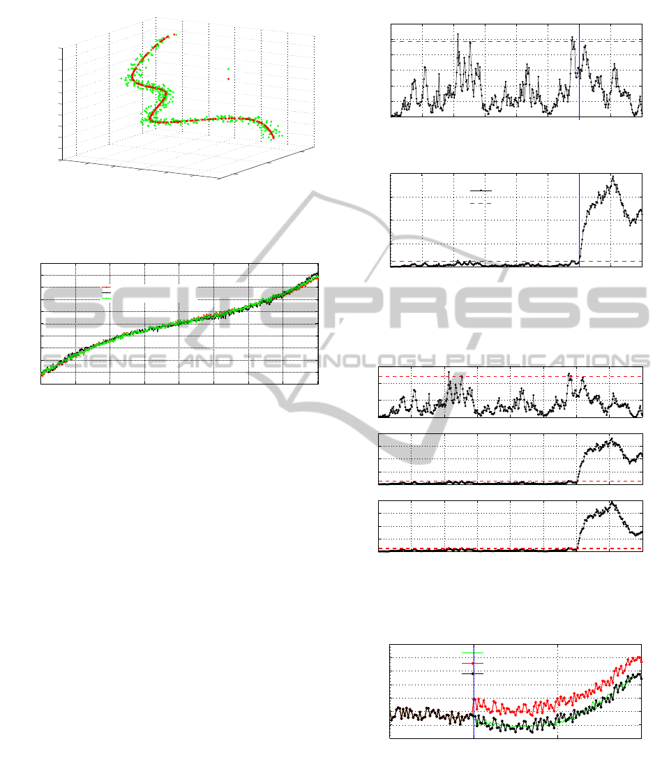
The estimated curve using the proposed NLPCA

model is shown in Fig.9. Fig.10 indicates the evo-

lution of the ﬁrst nonlinear principal component ob-

tained by three NLPCA models; the proposed model

(with 1-7-3 IT-Net structure, 3-8-1 RBF structure),

Verbeek algorithm (Hastie and Stuetzle, 1989) and

ﬁve-layer neural network (Hsieh and Li, 2001).

CombinedInputTrainingandRadialBasisFunctionNeuralNetworksbasedNonlinearPrincipalComponentsAnalysis

ModelAppliedforProcessMonitoring

489

0.5

−1.5

−1

−0.5

0.5

1.5

−1.5

−1

−0.5

0.5

1.5

2.5

3.5

Measurements

NLPCA IT-Net Estimation

Figure 9: Data and estimation by IT-Net for nonlinear sys-

tem

0 50 100 150 200 250 300 350 400

−2.5

−2

−1.5

−1

−0.5

0.5

1.5

2.5

Samples Number

NLPC

NLPC Obtained By Verbeeck

NLPC Obtained By Five Layers Neural Network

NLPC Obtained By IT−Net Neural Network

Figure 10: Evolution of the ﬁrst nonlinear principal compo-

nent.

For this example, Fig.11 represents the evolution

of SPE

in normal operating condition and in the

presence of a fault simulated on the variable x

from

sample 300 to 400. This fault is detected by this in-

dex.

Fig.12 indicates the time evolution of SPE

SPE

and SPE

indices after reconstruction of vari-

ables x

, x

and x

, respectively. The SPE

calcu-

lated after the reconstruction of x

is under its con-

trol limit which indicates that x

is the faulty vari-

able. Then we can reconstruct this variable in order

to give a replacement value for the faulty measure-

ments. Fig.13 shows, for variable x

, the fault free

measurements, the faulty measurements and the re-

placement values obtained by IT-Net and RBF neural

networks NLPCA model. It is clear, that the recon-

struction measurements are good estimations of fault

free measurements.

7 APPLICATION

The Tennessee Eastman (TECP) process shown in

Fig.14 is a simulation of a real plant, developed by

Downs and Vogel of the Eastman chemical Company

to provide a realistic simulation for evaluating process

0 50 100 150 200 250 300 350 400

x 10

−3

Samples number

SPE

0 50 100 150 200 250 300 350 400

0.02

0.04

0.06

0.08

Smples number

SPE

99% Control Limit

Figure 11: Fault detection for NLPCA IT-Net (a: SPE

plot

for normal operating conditions, b : SPE

plot with a simu-

lated fault on variable x

).)

0 50 100 150 200 250 300 350 400

x 10

−3

Filtered SPE after reconstruction of x

SPE

0 50 100 150 200 250 300 350 400

0.02

0.04

0.06

0.08

Filtered SPE after reconstruction of x

SPE

0 50 100 150 200 250 300 350 400

0.02

0.04

0.06

0.08

Filtered SPE after reconstruction of x

Sample Number

SPE

Figure 12: Fault isolation and faulty variable reconstruction

(a,b,c: SPE

plot after reconstruction each variable: x

, x

respectively.

250 300 350 400

0.2

0.4

0.6

0.8

1.2

Samples number

Faulty Variable Reconstruction

Faulty Variable

Free fault Variable

Figure 13: Faulty variable x

reconstruction.

control and monitoring methods, and widely used as

a source of data (Downs and Vogel, 1993), (Vogel,

1994).

The process has ﬁve major units: a reactor, a product

condenser, a vapor-liquid separator, a recycle com-

IJCCI2012-InternationalJointConferenceonComputationalIntelligence

490

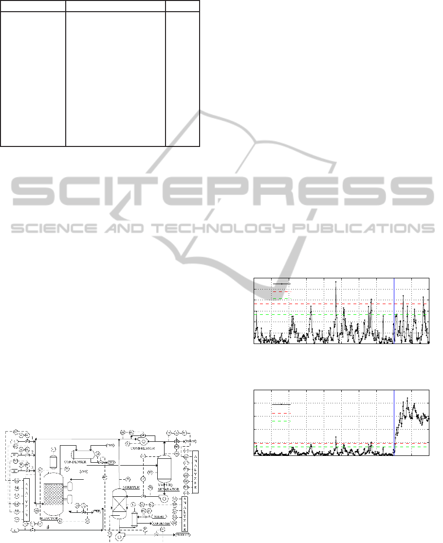
Table 1: Tennessee Eastman process Variables.

Measurements Variable name Units

D Feed Kg/h

E Feed Kg/h

A+C Feed kscmh

Reactor Feed Rate kscmh

Reactor Level %

Reactor Temp

◦

Product Sep Underﬂow m

/hr

Stripper underﬂow Kpa

Stripper Temp

◦

Steam Flow Kg/s

Reactor Cool Temp

◦

Cond Cool Temp

◦

pressor and product stripper. The process produces

products, G and H from four reactants A, C, D and E,

also presents an inert B, and by-product F.

The process here consists of 12 manipulated vari-

ables from the controller and 41 measurements, of

which 22 are continuous and 19 compositions mea-

sured by the Gaz chromatographic measurements can

not be collected continuously. In this paper only 12

continuous outputs are used in our study as demon-

strated in table 1.

There are two important factors that should be

considered, one is that the process is nonlinear, and

the second, the process operates in different modes

(Downs and Vogel, 1993), a 50:50 G:H mass ratio,

and others are in a 10:90 and a 90:10 G:H mass ra-

tio. Here, the process is operated in mode at 90:10

mass ratio. We generate a set of data according to this

condition. NLPCA is used to model the data. The

ﬁrst 400 samples are the normal data, and the next

100 samples involve data with a drift fault simulated

on the variable m

which mean that the relationship

among the process variables changes.

Figure 14: A diagram of the Tennessee Eastman and the

base control problem simulator.

Four (4) nonlinear principal components are re-

tained for the NLPCA model, which explains 98.68%

of the variance of data.

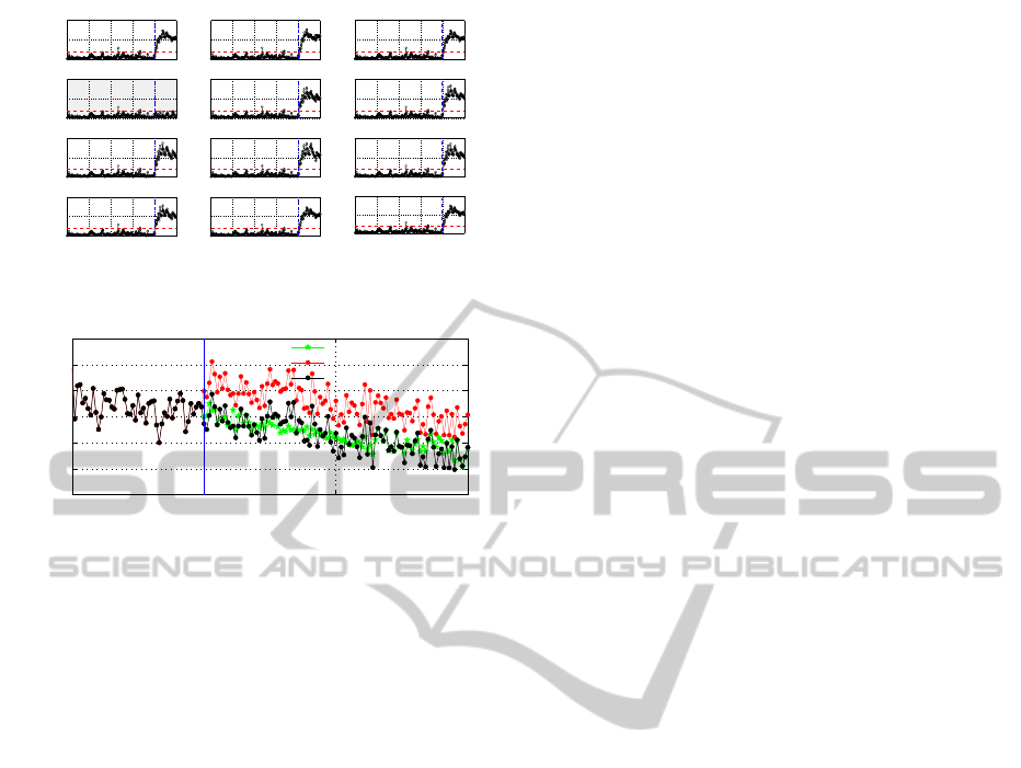
Based on the obtained NLPCA model, the indices

for detecting sensor faults and isolating faulty sensor

can be calculated on-line. Fig.15 shows time evolu-

tion of the squared prediction error SPE

for normal

operating conditions.

To apply the sensor data validationmethod (sensor

fault detection, isolation and reconstruction), a fault is

introduced for the variable m

between samples 400

and 500.

SPE

in 15 almost immediately allows to detect-

ing the fault. To identify sensor, a reconstruction ap-

proach is applied and SPE

f j

(j = 1, 2, ....12) are com-

puted. In Fig.17, the index SPE

(computed after

the reconstruction of m

) is under its control limit.

Which indicates that the faulty variable is m

. Vari-

able m

being identiﬁed as the faulty variable, then we

can reconstruct this variable in order to give a replace-

ment valuefor the faulty measurements. Fig.18 shows

the fault-free measurements, the faulty measurements

and the replacement values obtained by reconstruc-

tion for variable m

. It is clear that the reconstructed

measurements are good estimations of the fault-free

measurements.

0 50 100 150 200 250 300 350 400 450 500

0.005

0.01

0.015

0.02

0.025

0.03

Time

SPE

Control limit 99%

Control limit 95%

Figure 15: Time evolution of SPE

for normal condition.

0 50 100 150 200 250 300 350 400 450 500

0.02

0.04

0.06

0.08

0.1

Time

SPE

Control limit 99%

Control limit 95%

Figure 16: Time evolution of SPE

with a fault on variable

8 CONCLUSIONS

In this paper we have presented a new nonlinear

principal component analysis model. The proposed

NLPCA model is obtained by combining two cas-

cade neural networks. An RBF-Network for map-

CombinedInputTrainingandRadialBasisFunctionNeuralNetworksbasedNonlinearPrincipalComponentsAnalysis

ModelAppliedforProcessMonitoring

491

0 100 200 300 400 500

0.05

0.1

Samples number

SPE

0 100 200 300 400 500

0.05

0.1

Samples number

SPE

0 100 200 300 400 500

0.05

0.1

Samples number

SPE

0 100 200 300 400 500

0.05

0.1

Samples number

SPE

0 100 200 300 400 500

0.05

0.1

Samples number

SPE

0 100 200 300 400 500

0.05

0.1

Samples number

SPE

0 100 200 300 400 500

0.05

0.1

Samples number

SPE

0 100 200 300 400 500

0.05

0.1

Samples number

SPE

0 100 200 300 400 500

0.05

0.1

Samples number

SPE

0 100 200 300 400 500

0.05

0.1

Samples number

SPE

f10

0 100 200 300 400 500

0.05

0.1

Samples number

SPE

f11

0 100 200 300 400 500

0.05

0.1

Samples number

SPE

f12

Figure 17: Time evolution of SPE

after reconstruction of

each the variable m

350 400 450 500

Time

Reconstructed Measurements

Faulty Measurements

Fault Free Measurements

Figure 18: Reconstruction of the faulty measurements.

ping function and an IT-Net for demapping function.

The principal components are calculated using the

IT-Net which represent the demapping function, then

the RBF network is trained to perform the mapping

function. This two functions determines the NPLCA

model.

An NLPCA model is built, using data obtained

when the process is under normal condition. An ex-

tension of the nonlinear reconstruction approach is

proposed. The variable reconstruction consists in esti-

mating a variable from others process variables using

the NLPCA model, i.e. using the redundancy rela-

tions between this variable and the others. This ap-

proach is presented as an extension of the reconstruc-

tion in the linear case (Dunia et al., 1996) and leads to

an iterative expression of the reconstructed measure-

ments.

The proposed approach for sensor fault detection

and isolation, using nonlinear reconstruction method,

is presented and successfully applied to a Tennessee

Eastman process. The proposed approach also gives

replacement values of faulty measurements.

REFERENCES

Dong, D. and McAvoy, T. (1996). Nonlinear principal com-

ponent analysis based on principal curves and neural

networks. Computers and Chemical Engineering 20,

65 78.

Downs, J. and Vogel, E. (1993). A plant-wide industrial

control problem. Computers and chemical engineer-

ing Journal 17, 245-255.

Dunia, R., Qin, S., Ragot, J., and McAvoy, T. (1996). Iden-

tiﬁcation of faulty sensors using principal component

analysis. AIChE Journal 42, 2797-2812.

Harkat, M., Djellel, S., Doghmane, N., and Benouareth, M.

(2007). Sensor fault detection, isolation and recon-

struction using nonlinear principal component analy-

sis. Intarnational Journal of Automation and Comput-

ing, 4,.

Harkat, M., Mourot, G., and Ragot, J. (2003). Variable re-

construction using rbf-nlpca for process monitoring.

In IFAC Symposium on Fault Detection, Supervision

and Safety for Technical Process, SAFEPROCESS.

Washington, USA.

Hastie, T. and Stuetzle, W. (1989). Principal curves. Journal

of the American Statistical Association 84, 502-516.

Hsieh, W. and Li, C. (2001). Nonlinear principal component

analysis by neural networks. Tellus Journal 53A, 599-

615.

Kramer, M. (1991). Nonlinear principal component anal-

ysis using auto-associative neural networks. AIChE

Journal 37, 233-243.

LeBlanc, M. and Tibshirani, R. (1994). Adaptive principal

surfaces. Journal of American Statistical Association

89(425), 53-64.

Tan, S. and Mavrovouniotis, M. (1995). Reduction data

dimensionality through optimizing neural network in-

puts. AIChE Journal 41, 1471-1480.

Verbeek, J. (2001). A k-segments algorithm for ﬁnding

principal curves. IAS Technical Journal.

Vogel, N. R. E. (1994). Optimal steady-state operation of

the tennessee eastman challenge process. Computers

and chemical engineering Journal 19, 949-959.

Webb, A., Vlassis, N., and Krose, B. (1999). A loss function

to model selection in nonlinear principal components.

Neural Networks Journal 12, 339-345.

Zhu, Q. and Li, C. (2006). Dimensionality reduction with

input training neural network and its application in

chemical process modeling. Chinese Journal.

IJCCI2012-InternationalJointConferenceonComputationalIntelligence

492