A Comparison Study of Some Configurations of the Uninorm
Morphological Edge Detector
Manuel Gonz
´
alez-Hidalgo, Sebasti
`
a Massanet, Arnau Mir and Daniel Ruiz-Aguilera
Dept. of Mathematics and Computer Science, University of the Balearic Islands, Crta. Valldemossa Km. 7.5, Palma, Spain
Keywords:
Edge Detection, Fuzzy Mathematical Morphology, Uninorms, Fuzzy Implications, Hysteresis.
Abstract:
In this paper, we study the performance of the edge detector from the fuzzy mathematical morphology based on
conjunctive uninorms. Several different pairs of uninorm and fuzzy implication (configurations) are considered
in the fuzzy morphological gradient. The results are compared using an objective edge detection performance
measure, the so-called Pratt’s figure of merit. To reinforce the analysis a K-means clustering algorithm has
been applied to study the relation between the configurations and to determine which uninorm and implication
have to be chosen to obtain an optimal edge detector. According to the analysis of the obtained results, the
idempotent uninorm obtained using the classical negation, and its residual implication is the best configuration
in this framework.
1 INTRODUCTION
Edge detection is a fundamental low-level operation
in image processing, that is essential to develop high-
level operations such as segmentation, computer vi-
sion and recognition. Its performance is crucial for
the final results of the image processing technique.
In recent decades, a large number of edge detection
algorithms have been developed. These different ap-
proaches vary from classical algorithms (Pratt, 2007)
based on the use of a set of convolution masks, to new
techniques based on fuzzy sets and their extensions
(Bustince et al., 2009).
Among the fuzzy approaches, we can highlight
the fuzzy mathematical morphology that generalizes
the binary morphology (Serra, 1988) using concepts
and techniques of the fuzzy set theory (see (Bloch
and Ma
ˆ
ıtre, 1995), (Nachtegael and Kerre, 2000)).
This theory allows a better treatment and a more flex-
ible representation of the uncertainty and ambiguity
present in every level of an image. Morphological op-
erators are the basic tools of this theory. A morpho-
logical operator P transforms an image A to be anal-
ysed in a new image P(A,B) by means of an structur-
ing element B. The four basic morphological opera-
tions are dilation, erosion, opening and closing. Since
gray-level images can be represented as fuzzy sets,
fuzzy tools can be used to define fuzzy morphologi-
cal operators. This approach was introduced by De
Baets in (De Baets, 1997) and (De Baets, 2000) esta-
blishing a general framework where fuzzy morpho-
logical operators are defined using conjunctions and
fuzzy implications. The first step was based on the use
of t-norms in [0, 1] as conjunctions and their residual
implications as fuzzy implications. After analysing
which properties must satisfy the t-norm and the im-
plication to generate a fuzzy mathematical morphol-
ogy with all the desirable algebraical properties, it
was concluded that the couple formed by a nilpotent t-
norm and its residual implication generates a “good”
fuzzy mathematical morphology. Since nilpotent t-
norms are conjugates of the Łukasiewicz t-norm T
LK
,
this t-norm and its residual implication, that is the
Łukasiewicz implication I
LK
, are usually chosen to
define the fuzzy morphological operators of this the-
ory. Recently, it has been introduced a fuzzy math-
ematical morphology based on discrete t-norms with
good results in applications (Gonz
´
alez-Hidalgo et al.,
2010) using the fact that gray-level images are rep-
resented in fact as Z
2
→ L functions, where L is a
finite chain containing the gray-level values and not
as R
2
→ [0,1] functions.
However, other classes of conjunctions have been
used. In particular, the use of conjunctive uninorms
and their residual implications have been recently
proposed leading to a new fuzzy morphology that im-
proves the results in some applications, specially in
edge detection and noise removal (Gonz
´
alez-Hidalgo
et al., 2009b).
Focusing on edge detection purposes, the fuzzy
410
González-Hidalgo M., Massanet S., Mir A. and Ruiz-Aguilera D..
A Comparison Study of Some Configurations of the Uninorm Morphological Edge Detector.
DOI: 10.5220/0004148804100419
In Proceedings of the 4th International Joint Conference on Computational Intelligence (FCTA-2012), pages 410-419
ISBN: 978-989-8565-33-4
Copyright
c
 2012 SCITEPRESS (Science and Technology Publications, Lda.)

morphology must satisfy the extensivity and the anti-
extensivity of the erosion. This is the key property
for defining an edge detector based on the fuzzy mor-
phological gradient. Taking into account that the pair
(T
LK
,I
LK
) is the representative of the configurations
which define fuzzy morphological operators satisfy-
ing all the desirable algebraical properties, this con-
figuration has been widely used to implement the
edge detector of the fuzzy morphology based on t-
norms.
However, the mentioned property is satisfied with
some minimal properties of the structuring element,
the t-norm and the implication. Thus in (Gonz
´
alez-
Hidalgo et al., 2012) many more t-norms and impli-
cations were used to define a morphological gradi-
ent useful to detect edges. There, it was proved that
the pair (T
LK
,I
LK
) was the worst of the 40 considered
configurations, while (T
nM
,I
KD
), where
T
nM
(x,y) =

0 if x + y ≤1,
min{x,y} otherwise,
and I
KD
(x,y) = max{1 −x,y}, was the best configu-
ration generating a notable edge detector.
The aim of this contribution is to perform a sim-
ilar study for the fuzzy morphology based on con-
junctive uninorms. Only some particular uninorms
with their residual implications have been considered
in the fuzzy morphological gradient of this approach,
but similarly to the case of t-norms, many more uni-
norms and fuzzy implications can be chosen to gener-
ate the gradient. Thus we want to determine the best
combination of uninorm and implication to define an
optimal edge detector in this morphology. The re-
sults will be objectively compared using Pratt’s figure
of merit, FoM (Pratt, 2007). To compute this mea-
sure, the edge image must be binarized and thinned
to obtain edges with one-pixel width. This condi-
tions are consistent with Canny’s restrictions, set out
in (Canny, 1986). Therefore, after obtaining the fuzzy
edge image using the fuzzy gradient, this image is
thinned using Non-Maxima Suppression (NMS), a
well-known thinning algorithm proposed by Canny,
and the recently introduced automatic hysteresis al-
gorithm based on determining a “zone of instability”
in the histogram proposed in (Medina-Carnicer et al.,
2011) to binarize the image.
The communication is organized as follows. In
Section 2, we recall the definitions of morphological
operators and fuzzy operators that define them. In
Section 3, we present the considered uninorms and
implications, and the algorithm developed for each
configuration. In the next section, the results are pre-
sented and analysed. Finally, we share the conclu-
sions and future work we want to develop.
2 PRELIMINARIES
Fuzzy morphological operators are defined using
fuzzy operators such as uninorms and implications.
More details on these logical connectives can be
found in (Fodor et al., 1997) and (Baczy
´
nski and Ja-
yaram, 2008), respectively.
Definition 1. A uninorm is a commutative, associa-
tive, non-decreasing function U : [0,1]
2
→ [0, 1] with
neutral element e ∈ (0,1), i.e., U(e,x) = U(x,e) = x
for all x ∈[0, 1].
A uninorm U such that U(0,1) = 0 is called con-
junctive and if U (0,1) = 1, then it is called disjunc-
tive.
Definition 2. A binary operator I : [0, 1]
2
→ [0,1]
is a fuzzy implication if it is decreasing in the first
variable, increasing in the second one and it satisfies
I(0,0) = I(1, 1) = 1 and I(1,0) = 0.
Thus, we can define the basic fuzzy morphologi-
cal operators such as dilation and erosion. From now
on, we will use the following notation: U denotes a
conjunctive uninorm, I an implication, A a gray-level
image, and B a gray-level structuring element.
Definition 3. The fuzzy dilation D
U
(A,B) and the
fuzzy erosion E
I
(A,B) of A by B are the gray-level
images defined by
D
U
(A,B)(y) = sup
x
U(B(x −y), A(x))
E
I
(A,B)(y) = inf
x
I(B(x −y),A(x)).
As we have already mentioned, the following
proposition ensures the extensivity of the fuzzy dila-
tion and the anti-extensivity of the fuzzy erosion with
some minimal properties.
Proposition 1. Let U be a conjunctive uninorm with
neutral element e ∈ (0,1), I an implication that sat-
isfies (NP
e
), i.e., I(e,y) = y for all y ∈ [0, 1] and B
a gray-level structuring element such that B(0) = e.
Then the following inclusions hold:
E
I
(A,B) ⊆ A ⊆ D
U
(A,B).
Thus, as in the case of classical morphology, the
difference between the fuzzy dilation and the fuzzy
erosion of a gray-level image, D
U
(A,B) \E
I
(A,B),
known as fuzzy gradient operator, can be used in edge
detection.
3 CONFIGURATIONS AND
ALGORITHM
According to Proposition 1, any conjunctive uni-
norm with neutral element e ∈ (0, 1) and any impli-
cation that satisfies (NP
e
) are adequate to define the
AComparisonStudyofSomeConfigurationsoftheUninormMorphologicalEdgeDetector
411

Table 1: Considered uninorms.
Formula Class
U
1
(x,y) =

min{x,y} if y ≤ 1 −x,
max{x,y} if y > 1 −x.
Idempotent
U
2
(x,y) =

xy
(1−x)(1−y)+xy
if (x,y) /∈ {(0,1), (0, 1)},
0 otherwise.
Representable
U
3
(x,y) =



max{x + y −
1
2
,0} if x,y ≤
1
2
,
min{x + y −
1
2
,1} if x,y ≥
1
2
,
min{x,y} otherwise.
U
min
U
4
(x,y) =







0 if y ≤
1
2
−x,
1 if y ≥
3
2
−x,
max{x,y} x,y ≥
1
2
and y <
3
2
−x,
min{x,y} otherwise.
U
min
U
5
(x,y) =

max{x,y} if x,y ≥
1
2
,
min{x,y} otherwise.
U
min
U
6
(x,y) =

min{x,y} if y ≤
√
1 −x
2
,
max{x,y} if y >
√
1 −x
2
.
Idempotent
fuzzy gradient. Until now, in this uninorm approach,
only two types of left-continuous conjunctive uni-
norms and their residual implications have been used.
Specifically, they are defined as follows:
• Representable uninorms: Let e ∈ (0, 1) and let
h : [0,1] → [−∞,∞] be a strictly increasing con-
tinuous function with h(0) = −∞, h(e) = 0 and
h(1) = ∞. Then U
h
(x,y) =
=

h
−1
(h(x) + h(y)) if (x,y) /∈ {(1, 0), (0,1)},
0 otherwise,
is a conjunctive representable uninorm with neu-
tral element e, and its residual implication I
U
h
is
given by I
U
h
(x,y) =
=

h
−1
(h(y) −h(x)) if (x,y) /∈ {(0, 0), (1,1)},
1 otherwise.
• A specific type of idempotent uninorms. Let N be
a strong negation. The function given by
U
N
(x,y) =

min{x,y} if y ≤ N(x),
max{x,y} otherwise,
is a conjunctive idempotent uninorm. Its residual
implication is given by
I
U
N
(x,y) =

min{N(x),y} if y < x,
max{N(x),y} if y ≥x.
These two types of conjunctive uninorms guar-
antee most of the good algebraic and morphologi-
cal properties associated with the morphological op-
erators obtained from them (see (Gonz
´
alez-Hidalgo
et al., 2009a)). Note that from these conjunctive uni-
norms, their residual implications satisfy (NP
e
) since
any RU-implication
1
generated from a uninorm sat-
isfies (NP
e
) (see Proposition 5.4.2 in (Baczy
´
nski and
Jayaram, 2008)). However, this property is not rare
among the types of implications derived from uni-
norms, in fact it is also satisfied by the recently intro-
duced (h,e)-implications as proves Proposition 9 in
(Massanet and Torrens, 2011). This class of implica-
tions is generated by a continuous and strictly increas-
ing function h : [0,1] → [−∞,∞] with h(0) = −∞,
h(e) = 0 and h(1) = ∞ as follows:
I
h,e
(x,y) =



1 if x = 0,
h
−1

x
e
·h(y)

if x > 0 and y ≤ e,
h
−1

e
x
·h(y)

if x > 0 and y > e.
Consequently, we have considered the conjunctive
uninorms collected in Table 1 and the implications in
Table 2. Six uninorms have been considered. U
1
and
U
6
are the idempotent uninorms U
N
C
where N
C
(x) =
1 − x for all x ∈ [0,1] and U
N
2
, where N
2
(x) =
√
1 −x
2
, respectively. Moreover, U
2
is the repre-
sentable uninorm U
h
with h(x) = ln

x
1−x

. U
1
and U
2
have been already used in (Gonz
´
alez-Hidalgo et al.,
2009a). The rest of the considered uninorms belong
to the class of U
min
. This class allows us to choose a
uninorm with some desired underlying t-norm T and
t-conorm S in the following way U
T,S,e
(x,y) =
=



e ·T

x
e
,
y
e

if x,y ∈ [0,e],
e + (1 −e) ·S

x−e
1−e
,
y−e
1−e

if x,y ∈ [e,1],
min{x,y} otherwise.
Thus we have considered U
3
, U
4
and U
5
as
the uninorms of the class of U
min
given by
1
Given a a conjunctive uninorm U, its RU-implication is
defined by I(x, y) = sup{t ∈ [0,1]|U(x,t) ≤ y}.
IJCCI2012-InternationalJointConferenceonComputationalIntelligence
412

Table 2: Considered implications.
Formula Class
I
1
(x,y) =

max{1 −x, y} if x ≤y,
min{1 −x, y} if x > y.
RU-implication
I
2
(x,y) =
(
(1−x)y
x+y−2xy
if (x,y) /∈ {(0,0), (1, 1)},
1 otherwise.
RU-implication
I
3
(x,y) =







1
2
+ y −x if (y < x <
1
2
) or (y > x ≥
1
2
),
1
2
if x ≥y ≥
1
2
,
1 if x ≤ y <
1
2
,
y otherwise.
RU-implication
I
4
(x,y) =











1 if y = 1 or x ≤y <
1
2
,
max{
1
2
−x,y} if y < x <
1
2
,
3
2
−x if
1
2
≤ x ≤y and y >
3
2
−x,
1
2
if
1
2
≤ y < x,
y otherwise.
RU-implication
I
5
(x,y) =







y if
1
2
≤ x < y,
1
2
if
1
2
≤ y ≤ x,
1 if x ≤y <
1
2
,
y otherwise.
RU-implication
I
6
(x,y) =









1 if x = 0,
y
2x
(1−y)
2x
+y
2x
if x > 0, y ≤
1
2
y
1
2x
(1−y)
1
2x
+y
1
2x
otherwise.
(h,e)-implication
I
7
(x,y) =

max{
√
1 −x
2
,y} if x ≤ y,
min{
√
1 −x
2
,y} if x > y.
RU-implication
U
T
LK
,S
LK
,
1
2
, U
T
nM
,S
nM
,
1
2
and U
T
M
,S
M
,
1
2
, respectively,
where T
LK
(x,y) = max{x + y − 1,0}, T
M
(x,y) =
min{x,y},
T
nM
(x,y) =

0 if x + y ≤1,
min{x,y} otherwise,
and S
LK
, S
M
and S
nM
are their N
C
-dual t-conorms, re-
spectively (see (Klement et al., 2000) for more de-
tails). All the uninorms have neutral element e =
1
2
except U
6
, with neutral element e =
√
2
2
.
On the other hand, we have considered 7 fuzzy
implications. Six of them, from I
1
to I
5
and I
7
, are in
the same order the residual implications of the con-
sidered uninorms. Finally, I
6
is the (h,e)-implication
generated by h(x) = ln

x
1−x

. All these implications
satisfy (NP
e
) with e =
1
2
, except I
7
that satisfies it with
e =
√
2
2
. Thus 31 different configurations of uninorm
and implications can be considered in the fuzzy gra-
dient since U
6
and I
7
must be applied together.
3.1 NMS and Automatic Hysteresis
To compare the results, we need some objective per-
formance measure on edge detection. These measures
require, in addition to the binary edge image with
edges of one pixel width (DE) obtained by the edge
detector we want to evaluate, a reference edge image
or ground truth edge image (GT) which is a binary
edge image with edges of one pixel width containing
the real edges of the original image. There are several
measures of performance for edge detection in the lit-
erature, see (Papari and Petkov, 2011). In this paper
we are going to use the measure proposed by Pratt,
Pratt’s figure of merit, to quantify the similarity be-
tween (DE) and (GT). This measure is defined by
FoM =
1
max{card{DE},card{GT }}
·
∑
x∈DE
1
1 + ad
2
,
where card is the number of edge points of the image,
a is a scaling constant and d is the separation distance
of an actual edge point to the ideal edge points. In our
case, we considered a = 1 and the Euclidean distance
d. A higher value of FoM indicates a better capability
to detect edges.
AComparisonStudyofSomeConfigurationsoftheUninormMorphologicalEdgeDetector
413

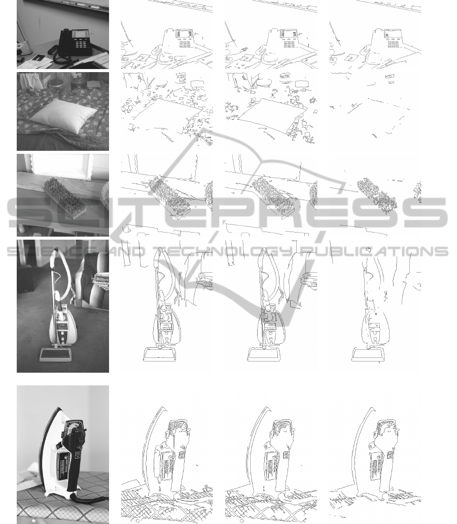
(a) Input original image. (b) Fuzzy edge image obtained
with the fuzzy gradient.
(c) NMS. (d) Output binary thin edge image.
Figure 1: Sequence of the proposed algorithm.
However, the fuzzy based edge detectors gener-
ate an image where the value of a pixel represents its
membership degree to the set of edges. This idea con-
tradicts the restrictions of Canny (Canny, 1986), forc-
ing a representation of the edges as binary images of
one pixel width. Therefore the fuzzy edge image must
be thinned and binarized. The fuzzy edge image will
contain large values where there is a strong image gra-
dient, but to identify edges the broad regions present
in areas where the slope is large must be thinned so
that only the magnitudes at those points which are lo-
cal maxima remain. NMS performs this by suppress-
ing all values along the line of the gradient that are not
peak values (see (Canny, 1986)). NMS has been per-
formed using P. Kovesis’ implementation in Matlab
(Kovesi, 2012).
Finally, to binarize the image, we have im-
plemented an automatic, non-supervised, hysteresis
based on the determination of the instability zone of
the histogram to find the thresholds (see (Medina-
Carnicer et al., 2011)). Hysteresis allows to choose
which pixels are relevant in order to be selected as
edges, using their membership values. Two threshold
values T
1
, T
2
with T
1
≤ T
2
are used. All the pixels
with a membership value greater than T
2
are consid-
ered as edges, while those which are lower to T
1
are
discarded. Those pixels whose membership value is
between the two values are selected if and only if they
are connected with other pixels above T
2
. The method
needs some initial set of candidates for the threshold
values. In this case, {0.01,. . . ,0.25} has been intro-
duced, the same set used in (Medina-Carnicer et al.,
2011). In Figure 1, the sequence of the algorithm is
displayed.
4 RESULTS AND ANALYSIS
The comparison method explained in the previous
section needs an image database containing, in ad-
dition of the original images, their corresponding
ground truth edge images in order to compare the out-
puts obtained by the different configurations. Thus,
we have used the original images and their ground
truth edge images of the public image database of the
University of South Florida
2
(Bowyer et al., 1999).
In this stage of our study, we have used 15 out of the
50 images of the database.
The results, obtained all of them using the follow-
ing isotropic structuring element scaled by e, the neu-
tral element of the uninorm,
B = e ·


0.86 0.86 0.86
0.86 1 0.86
0.86 0.86 0.86


which had been already used in (Nachtegael and
Kerre, 2000), are summarized in Table 3. We have set
the previous structuring element because it provides
the best results with most of the configurations of the
fuzzy gradient. However, we are aware that the results
may differ if we change the structuring element. In
the table, we compute some statistical measures asso-
ciated to the obtained FoM values. For example, the
mean value is the mean of the obtained FoM values
using a particular configuration in the fuzzy gradient
for the 15 considered images. As it can be observed,
the most significant fact is the dependence of the elec-
tion of the pair uninorm-implication into the results.
Note that although some of the configurations obtain
quite similar results, for example (U
4
,I
1
) and (U
4
,I
6
),
the difference between the results obtained using the
best configuration, that is (U
1
,I
1
), with respect to the
worst one (U
3
,I
3
) is notable, a gap of 0.1644. The
worst configuration according to its mean value is also
the worst configuration for 12 of these images. On the
other hand, the configuration with the highest mean
value is not the configuration with the highest num-
ber of images for which a particular configuration is
the best one of the 31 considered configurations, that
is shared by (U
1
,I
4
) and (U
1
,I
5
). This is because the
standard deviation of the FoM values obtained using
(U
1
,I
1
) is lower than the one obtained using these two
configurations, i.e., (U
1
,I
1
) is more stable. In Figure
2, we show some of the edge images obtained using
some of these configurations. Note that the visual re-
sults agree with the FoM values since the results ob-
tained by (U
3
,I
3
) contain, in general, few edges with
respect to the others. Note that the presence of I
1
or
2
It can be downloaded from ftp://figment.csee.usf.edu/
pub/ROC/edge comparison dataset.tar.gz
IJCCI2012-InternationalJointConferenceonComputationalIntelligence
414

Table 3: Statistical measures associated to obtained FoM values.
Configuration
Mean Std. Dev.
Images Configuration
Mean Std. Dev.
Images
Unin. Imp. X × Unin. Imp. X ×
U
1
I
1
0.4588 0.0911 2 0
U
2
I
1
0.4406 0.0960 0 0
I
2
0.4416 0.0883 0 0 I
2
0.4060 0.1088 1 0
I
3
0.4295 0.0926 0 0 I
3
0.3953 0.1074 1 0
I
4
0.4483 0.1004 4 0 I
4
0.4314 0.0947 1 0
I
5
0.4482 0.1006 4 1 I
5
0.4317 0.0941 1 0
I
6
0.4545 0.0925 3 0 I
6
0.4351 0.0854 1 0
U
3
I
1
0.4145 0.0849 0 0
U
4
I
1
0.4218 0.0787 0 0
I
2
0.3682 0.1096 0 0 I
2
0.3807 0.1114 0 0
I
3
0.2944 0.1127 1 12 I
3
0.3089 0.1206 0 1
I
4
0.3584 0.0902 0 0 I
4
0.3645 0.0916 0 0
I
5
0.3583 0.0903 0 0 I
5
0.3646 0.0916 0 0
I
6
0.4146 0.0812 0 0 I
6
0.4218 0.0786 0 0
U
5
I
1
0.4218 0.0787 0 0 U
6
I
7
0.4417 0.0905 0 0
I
2
0.3807 0.1114 0 0
I
3
0.3090 0.1207 0 1
I
4
0.3645 0.0916 0 0
I
5
0.3546 0.0916 0 0
I
6
0.4218 0.0786 0 0
I
6
in a given configuration improves the results. An-
other fact to highlight is the similarity of the results
obtained using U
4
and U
5
with a fixed implication.
This is due to the similar expressions in a certain re-
gion of both uninorms and the choice of structuring
element B. Finally, in Figure 3, the best configuration
and the worst one for some images according to FoM
are displayed.
To reinforce the previous analysis, a clustering
method has been applied to study the relations be-
tween the configurations. Firstly, we have determined
the optimal number of clusters according to the so-
called F-test of variability reduction, leading to 4 clus-
ters. Finally, applying the K-means algorithm with
this number of clusters we have obtained the follow-
ing results:
• Cluster 1: U
1
with I
1
−I
6
, U
2
with I
1
, I
4
−I
6
, U
3
−
U
5
with I
1
and I
6
, U
6
with I
7
.
• Cluster 2: U
2
with I
2
and I
3
, U
3
−U
5
with I
2
.
• Cluster 3: U
3
−U
5
with I
4
and I
5
.
• Cluster 4: U
3
−U
5
with I
3
.
These clusters allow us to set up a certain perfor-
mance ranking with the considered logical operators:
U
1
,U
6
U
2
U
3
,U
4
,U
5
,
I
1
,I
6
,I
7
 I
2
,I
4
,I
5
 I
3
,
where A,B C indicates that those configurations ob-
tained from A or B give better results than those ob-
tained from C.
From this ranking, some remarks can be stated:
1. Idempotent and representable uninorms generate
better edge detectors than uninorms of the class
U
min
.
2. The worst implication is I
3
, that is the resid-
ual implication of the uninorm U
T
LK
,S
LK
,
1
2
. This
fact is coherent with the bad behaviour of the
Łukasiewicz t-norm in the morphology based on
t-norms in [0,1].
3. The (h,e)-implication I
7
gives competitive results
and therefore, the role of this class of implications
in fuzzy morphology should be seriously investi-
gated.
In Figure 4, these remarks can be graphically ob-
served. In both subfigures, the vertical axis corre-
spond to the mean of the FoM values of each con-
figuration, while the horitzontal ones of Figure 4-(a)
correspond to the different considered uninorms and
analogously the different considered implications in
Figure 4-(b). A dotted point is associated to the FoM
value mean of a configuration (U
i
,I
j
).
5 CONCLUSIONS AND FUTURE
WORK
In this work, a comparison of morphological gradi-
ents generated from different configurations of uni-
norm and fuzzy implication has been performed
showing that the configuration (U
1
,I
1
) where U
1
is
AComparisonStudyofSomeConfigurationsoftheUninormMorphologicalEdgeDetector
415

(a) Original image. (b) (U
1
,I
1
). (c) (U
2
,I
6
). (d) (U
3
,I
3
).
Figure 2: Some edge images obtained with different configurations.
the idempotent uninorm obtained from the classical
negation and I
1
is its residual implication is the best
configuration according to the performance measure
on edge detection FoM. It has been shown that analo-
gously to what happens on the morphology based on
t-norms, the uninorms generated in some region by
the Łukasiewicz t-norm give bad results, both from
the visual point of view and the FoM values obtained
by the edge images. In addition, we have proved the
possible use of the new class of implications, (h, e)-
IJCCI2012-InternationalJointConferenceonComputationalIntelligence
416

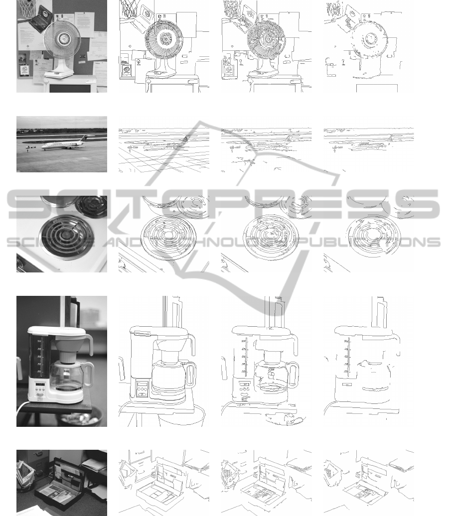
(a) Original image. (b) Ground truth. (c) (U
1
,I
4
). (d) (U
3
,I
3
).
(e) Original image. (f) Ground truth. (g) (U
1
,I
6
). (h) (U
3
,I
3
).
(i) Original image. (j) Ground truth. (k) (U
1
,I
4
). (l) (U
3
,I
3
).
(m) Original image. (n) Ground truth. (o) (U
1
,I
1
). (p) (U
3
,I
3
).
(q) Original image. (r) Ground truth. (s) (U
2
,I
4
). (t) (U
3
,I
3
).
Figure 3: Best (3rd column) and worst (4th column) edge images obtained with the considered configurations according to
their FoM value.
implications, in image processing applications.
In the future work, we want to to increase the num-
ber of images for the comparison including all the im-
ages in the used database. The next step would be the
comparison of the uninorm edge detector generated
by (U
1
,I
1
) with some classical edge detectors such
as Canny, Sobel, Prewitt, etc. In addition, we want
to generalize the morphological operators using a t-
AComparisonStudyofSomeConfigurationsoftheUninormMorphologicalEdgeDetector
417

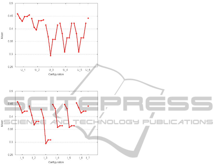
(a) Comparison according to uninorms.
(b) Comparison according to implications.
Figure 4: Graphical comparison of the performance of the
considered uninorms (a) and implications (b).
conorm and a t-norm rather than the operations sup
and inf respectively in the dilation and erosion. As
the maximum is the smallest of the t-conorms and the
minimum is the largest of the t-norms, this generaliza-
tion could improve the results since it would extend
the morphological gradient allowing a greater detec-
tion of edges.
ACKNOWLEDGEMENTS
This work has been partially supported by the national
project MTM2009-10320 with FEDER funds.
REFERENCES
Baczy
´
nski, M. and Jayaram, B. (2008). Fuzzy Implications,
volume 231 of Studies in Fuzziness and Soft Comput-
ing. Springer, Berlin Heidelberg.
Bloch, I. and Ma
ˆ
ıtre, H. (1995). Fuzzy mathematical mor-
phologies: a comparative study. Pattern Recognition,
28:1341–1387.
Bowyer, K., Kranenburg, C., and Dougherty, S. (1999).
Edge detector evaluation using empirical ROC curves.
Computer Vision and Pattern Recognition, 1:354–359.
Bustince, H., Barrenechea, E., Pagola, M., and Fernandez,
J. (2009). Interval-valued fuzzy sets constructed from
matrices: Application to edge detection. Fuzzy Sets
and Systems, 160(13):1819–1840.
Canny, J. (1986). A computational approach to edge de-
tection. IEEE Trans. Pattern Anal. Mach. Intell.,
8(6):679–698.
De Baets, B. (1997). Fuzzy morphology: A logical ap-
proach. In Ayyub, B. M. and Gupta, M. M., ed-
itors, Uncertainty Analysis in Engineering and Sci-
ence: Fuzzy Logic, Statistics, and Neural Network Ap-
proach, pages 53–68. Kluwer Academic Publishers,
Norwell.
De Baets, B. (2000). Generalized idempotence in fuzzy
mathematical morphology. In Kerre, E. E. and
Nachtegael, M., editors, Fuzzy techniques in image
processing, number 52 in Studies in Fuzziness and
Soft Computing, chapter 2, pages 58–75. Physica-
Verlag, New York.
Fodor, J., Yager, R., and Rybalov, A. (1997). Structure of
uninorms. Int. J. Uncertainty, Fuzziness, Knowledge-
Based Systems, 5:411–427.
Gonz
´
alez-Hidalgo, M., Massanet, S., and J.Torrens (2010).
Discrete t-norms in a fuzzy mathematical morphol-
ogy: Algebraic properties and experimental results.
In Proceedings of WCCI-FUZZ-IEEE, pages 1194–
1201, Barcelona, Spain.
Gonz
´
alez-Hidalgo, M., Massanet, S., and Mir, A. (2012).
Determining the best pair of t-norm and implication
in the morphological gradient. In Proceedings of XVI
Congreso Espa
˜
nol sobre Tecnolog
´
ıas y L
´
ogica Fuzzy
(ESTYLF), pages 510–515, Valladolid, Spain. (In
Spanish).
Gonz
´
alez-Hidalgo, M., Mir-Torres, A., Ruiz-Aguilera,
D., and Torrens, J. (2009a). Edge-images using
a uninorm-based fuzzy mathematical morphology:
Opening and closing. In Tavares, J. and Jorge, N.,
editors, Advances in Computational Vision and Med-
ical Image Processing, number 13 in Computational
Methods in Applied Sciences, chapter 8, pages 137–
157. Springer, Netherlands.
Gonz
´
alez-Hidalgo, M., Mir-Torres, A., Ruiz-Aguilera, D.,
and Torrens, J. (2009b). Image analysis applications
of morphological operators based on uninorms. In
Proceedings of the IFSA-EUSFLAT 2009 Conference,
pages 630–635, Lisbon, Portugal.
Klement, E., Mesiar, R., and Pap, E. (2000). Triangular
norms. Kluwer Academic Publishers, London.
Kovesi, P. D. (2012). MATLAB and Octave functions for
computer vision and image processing. Centre for Ex-
ploration Targeting, School of Earth and Environment,
The University of Western Australia. Available from:
http://www.csse.uwa.edu.au/∼pk/research/matlabfns/.
IJCCI2012-InternationalJointConferenceonComputationalIntelligence
418

Massanet, S. and Torrens, J. (2011). On a new class of fuzzy
implications: h-implications and generalizations. In-
formation Sciences, 181(11):2111 – 2127.
Medina-Carnicer, R., Mu
˜
noz-Salinas, R., Yeguas-Bolivar,
E., and Diaz-Mas, L. (2011). A novel method to look
for the hysteresis thresholds for the Canny edge detec-
tor. Pattern Recognition, 44(6):1201 – 1211.
Nachtegael, M. and Kerre, E. (2000). Classical and fuzzy
approaches towards mathematical morphology. In
Kerre, E. E. and Nachtegael, M., editors, Fuzzy tech-
niques in image processing, number 52 in Studies in
Fuzziness and Soft Computing, chapter 1, pages 3–57.
Physica-Verlag, New York.
Papari, G. and Petkov, N. (2011). Edge and line oriented
contour detection: State of the art. Image and Vision
Computing, 29(2-3):79 – 103.
Pratt, W. K. (2007). Digital Image Processing. Wiley-
Interscience, 4 edition.
Serra, J. (1982,1988). Image analysis and mathematical
morphology, vols. 1, 2. Academic Press, London.
AComparisonStudyofSomeConfigurationsoftheUninormMorphologicalEdgeDetector
419