An Optimization Method for Training Generalized Hidden Markov
Model based on Generalized Jensen Inequality
Y. M. Hu
1
, F. Y. Xie
1,2
, B. Wu
1
, Y. Cheng
1
, G. F. Jia
1
, Y. Wang
3
and M. Y. Li
1
1
State Key Laboratory for Digital Manufacturing Equipment and Technology,
Huazhong University of Science and Technology, Wuhan 430074, P.R. China
2
School of Mechanical and Electronical Engineering, East China Jiaotong University, Nanchang 330013, P.R. China
3
Woodruff School of Mechanical Engineering, Georgia Institute of Technology, Atlanta, GA 30332-0405, U.S.A.
Keywords: Generalized Hidden Markov Model, Generalized Jensen Inequality, Generalized Baum-Welch Algorithm.
Abstract: Recently a generalized hidden Markov model (GHMM) was proposed for solving the problems of aleatory
uncertainty and epistemic uncertainty in engineering application. In GHMM, the aleraory uncertainty is
derived by the probability measure while epistemic uncertainty is modelled by the generalized interval.
Given any finite observation sequence as training data, the problem of training GHMM is often encountered.
In this paper, an optimization method for training GHMM, as a generalization of Baum-Welch algorithm, is
proposed. The generalized convex and concave functions based on the generalized interval are proposed for
inferring the generalized Jensen inequality. With generalized Baum-Welch’s auxiliary function and
generalized Jensen inequality, similar to the multiple observations training, the GHMM parameters are
estimated and updated by the lower and the bound observation sequences. A set of training equations and
re-estimated formulas have been derived by optimizing the objective function. Similar to multiple
observations (expectation maximization) EM algorithm, this method guarantees the local maximum of the
lower and the upper bound and hence the convergence of the GHMM training process.
1 INTRODUCTION
Jensen inequality, named Johan Jensen in 1906,
relates the value of a convex function of an integral
to the integral of the convex function (Jensen, 1906).
As an important mathematical tool it has been
widely used, such as probability density function,
statistical physics, information theory, and
optimization theory. However it does not
differentiate two kinds of uncertainties, namely,
aleatory uncertainty is inherent randomness, whereas
epistemic uncertainty is due to lack of knowledge.
Epistemic uncertainty is significant and cannot be
ignored. The generalized interval provides a valid
method for solving epistemic uncertainty. Compared
to the classical interval, generalized interval based
on the Kaucher arithmetic (Kaucher, 1980) is better
in algebraic properties so that the calculus can be
simplified (Wang, 2011).
As a generalization of hidden Markov model
(HMM) (Rabiner, 1989), the (Generalized hidden
Markov model) GHMM, which is based on the
generalized interval probability, are stochastic
models in capable of statistical learning and
classification (Wang, 2011). The optimization of
GHMM parameters is a crucial problem for the
application of GHMMs, since it can create the best
models for real phenomena. Similar to HMM, a
generalized Baum-Welch algorithm can be adapted
such that the result is the local maximum (Baum et
al., 1970).
In this paper, an optimization method, which is
for training GHMM based on the generalized jensen
inequality and the generalization Baum-Welch
algorithm, is proposed. The classical convex
functions, the classical concave functions, and the
Jensen inequality are respectively developed by the
use of generalized intervals. The parameters of
GHMM are estimated and updated through
generalized Baum-Welch algorithm. A generalized
Baum-Welch’s auxiliary function is built up and the
generalized Jensen inequality is used. Similar to the
multiple observations training in HMM (Li et al.,
2000), the GHMM parameters are estimated and
updated by given the lower and the bound
observation sequences. A set of training equations
268
M. Hu Y., Y. Xie F., Wu B., Cheng Y., F. Jia G., Wang Y. and Y. Li M..
An Optimization Method for Training Generalized Hidden Markov Model based on Generalized Jensen Inequality.
DOI: 10.5220/0004118202680274
In Proceedings of the 9th International Conference on Informatics in Control, Automation and Robotics (ICINCO-2012), pages 268-274
ISBN: 978-989-8565-21-1
Copyright
c
 2012 SCITEPRESS (Science and Technology Publications, Lda.)

have been derived by optimizing the objective
function. A set of GHMM re-estimated formulas has
been derived by the unique maximum of the
objective function. The proposed optimization
method takes advantage of the good algebraic
property in the generalized interval. This provides an
efficient approach to train the GHMM.
2 BACKGROUND
2.1 Generalized Interval
A generalized interval
: [ , ]xxx
, (
x,x 
) is
defined by a pair of real numbers as
x
and
x
(Popova,
2000, Gardenes, 2001). Let
: [ , ]xxx
,
0, 0xx
 
x,x 
and
: [ , ]yyy
,
0, 0yy
(
y,y 
) be interval variables, and let generalized
interval function be
     
[ , ]t f t f tf
(Markov,
1979), where
t
is a real variable, then, the arithmetic
operations of generalized intervals based on the
Kaucher arithmetic are follows.
+ =[ + , + ]x y x yxy
.
(1)
- =[ - , - ]daul x y x yxy
.
(2)
=[ , ]x y x y  xy
.
(3)
=[ , ]daul x y x y  xy
,
0, 0yy
.
(4)
log =[log ,log ]xxx
,
0, 0xx
.
(5)
     
d [ d , d ]t t f t t f t t
  
f
.
(6)
     
,d t dt d f t dt d f t dt



f
.
(7)
     
 
0
lim
x
t t t daul t t
x


    

f f f
(8)
The less than or equal to partial order
relationship between two generalized intervals is
defined as
[ , ] [ , ]x x y y x y x y    
.
(9)
2.2 Generalized Hidden Markov Model
The GHMM is a generalization of HMM in the
context of generalized interval probability theory.
The generalized interval probability is based on the
generalized interval with a form of probability. In
GHMM, all probability parameters of HMM are
replaced by the generalized interval probabilities.
The boldface symbols have generalized interval
values.
A GHMM is characterized as follows. The
values of hidden states are in the form of
12
{ , , , }
N
S S S S
, where N is the total number of
possible hidden states. The hidden state variable at
time t is
t
q
, where
: [ , ]
t t t
qqq
. The M possible
distinct observation symbols per state are
12
{ , , , }
M
V v v v
. The generalized observation
sequence is in the form of
 
12
, , ,
T
O o o o
where
t
o
is the observation value at time t. Note that the
observations have the values of generalized intervals.
Equivalently the lower bound sequence
 
12 T
O o ,o , o
and upper bound sequence can be
viewed separately, where, the value of
t
o
and
t
o
(t=1,…,T) can be any of
12
{ , , , }
M
v v v
.
Let
pro[ , ]
t t t
q q q
and
pro[ , ]
t t t
o o o
be real-
valued random variables.
 
ij
NN
Aa
is the state
transition interval probability matrix,
 
1ij t j t i
q S |q S

  pa
,
(1 )i, j N
is the
interval probability of the transition from state
i
S
at
time t to state
j
S
at time t+1.
 
()
j
NM
k

Bb
is the
observation interval probability matrix.
 
 
|
j t k t j
k o v q S  pb
,
 
1 ,1j N k M   
is the interval probability of observations in state
j
S
at time t.
 
1
i
N
π π
is the initial state interval
probability distribution,
 
1ii
qSp 
,
 
1 iN
.
The compact GHMM is denoted as
 
λ A,B,π
.
Similar to classical HMM, the GHMM is usually
used to solve three basic problems in real
applications. The training problem of the GHMM is
the crucial one. Its goal is to optimize the model
parameters so that we can obtain best models for real
phenomena. The proposed generalized Baum-Welch
algorithm, as a generalization of Baum-Welch
algorithm in the context of the generalized interval
probability, provides an efficient approach to train
GHMM. The generalized Baum-Welch algorithm is
based on the generalized Jensen inequality which is
introduced in the following section.
An Optimization Method for Training Generalized Hidden Markov Model based on Generalized Jensen Inequality
269

3 GENERALIZED JENSEN
INEQUALITY
3.1 Generalized Convex Function
Following the definition of interval function by
Markov, a generalized convex function is defined as
following (Markov, 1979)
A generalized interval function
 
tf
is in the
domain of the generalized interval , where
t
is a
real variable,
12
,tt
if
     
1 1 2 2 1 1 2 2
+t t t tf r r rf r f
(10)
Where
1
1
1
: [ , ]rrr
,
2
2
2
: [ , ]rrr
,
1
1
0, 0rr
,
2
2
0, 0rr
, and
12
[1,1]rr
.
 
tf
is named as
generalized convex function in the generalized
interval .
Under the same assumption condition as
generalized convex function, if
     
1 1 2 2 1 1 2 2
+t t t tf r r rf r f
(11)
 
tf
is named as generalized concave function in
the generalized interval , especially, when
 
logttf
(t>0), then,
 
2
2
2
0
dt
t
dt
  
f
,
 
tf
is
named as a strict generalized concavity of log
function.
3.2 Generalized Jensen Inequality
For a generalized convex function
 
tf
, numbers
12
, , ,
n
t t t…
in its domain, and
:=[ , ]
i
i
i
rrr
,
0, 0
i
i
rr
( 1,2, , )in …
,
1
= [1,1]
n
i
i

r
, the
generalized Jensen inequality can be stated as
 
11
nn
i i i i
ii
tt






f r rf
(12)
A mathematical induction is adopted to prove
formula (12).
Proof. When n=2, formula (12) is a defined form of
generalized convex function, thus it is correct.
If n=k,
 
11
kk
i i i i
ii
tt






f r rf
now we need to prove
that formula (12) is also correct when n=k+1
 
1
1
1
1
11
1
11
( ) ( )
k
ii
i
k
kk
i i k k k k
i
k k k k
t
t t t
dual dual












   








fr
rr
f r r r
r r r r
 
   
1
1
11
1
11
1
11
1
1
1
()
( ) ( )
()
( ).
k
kk
i i k k k k
i
k k k k
k
i i k k k k
i
k
ii
i
t t t
dual dual
t t t
t











   



  




rr
rf r r f
r r r r
rf r f r f
rf
Thus, we can obtain that formula (12) is correct for
all i
( 1,2, , )in …
.
It is a simple corollary that the opposite is true
for generalized concave function transformations,
the generalized interval formula is
 
11
nn
i i i i
ii
tt






f r rf
(13)
4 OPTIMIZATION METHOD IN
TRAINING PROCESS OF A
GHMM
The training problem of GHMM is that given the
observation sequence
 
12 T
, , ,O o o o…
, we adjust
the model parameters
A,B,π
to maximize the lower
and the upper bound of
()|p O λ
. Similar to the
training of HMM, we can choose
 
λ A,B,π
so
that the lower and the upper bound of
()|p O λ
are
both locally maximized by using an iterative
procedure of the generalized Baum-Welch algorithm.
The optimization method is based on the following
two lemmas similar to inference of HMM re-
estimation formulas (Levinson et al., 1983).
Lemma 1: Let
:[ , ]
i
ii
uuu
,
0, 0, 1, ,
i
i
u u i S  
be positive interval real numbers, and let
:[ , ]
i
ii
vvv
,
0, 0, 1, ,
i
i
v v i S  
be nonnegative
interval real numbers such that
[0,0]
i
i


v
. Then
from the generalized concavity of the log function
and the generalized Jensen inequality, it follows that
 
log .log
1
. log log
i
i i i
i
i k i
ik
i i i i
i
k
k
dual dual dual
dual
dual















v
uv
u u u
u v u u
u
(14)
ICINCO 2012 - 9th International Conference on Informatics in Control, Automation and Robotics
270

Here every summation is from 1 to S.
Lemma 2: If
0, 1, ,
i
iNc
, then subject to the
constraint
1
1
N
i
i
t



, the generalized interval function
is
 
1
log
N
ii
i
tt



f c
(15)
We can obtain its unique global maximum when
1
N
i i i
i
t dual



cc
(16)
The proof of formulas (16) is similar to Lagrange
method (Levinson et al., 1983)
 
0
i
i
i
ii
t dual t
x dualx


   




f
c

(17)
Multiplying by
i
t
and summing over i, we can obtain
i
i
c


, so formula (16) can be derived.
4.1 Auxiliary Interval Function
In order to train the GHMM, the lower bound
observation sequence
 
12 T
O o ,o , o
, for
example, is used as the input of auxiliary interval
function
 
,
l
Q 
, which is defined as following.
Let
l
i
u
be the joint interval probability
 
: , |
l
i
O puQ 
which is depended on model

,
and let
l
i
v
be the same joint interval probability
 
: , |
l
i
O pvQ 
which is depended on model

,
where
 
12
, , ,
T
Q q q q
, then
 
|
l
i
i
O

pu 
,
 
|
l
i
i
O

pv 
(18)
Let auxiliary interval function
 
,
l
Q 
(Levinson et
al., 1983) be
 
 
 
, , | log , |
l
OO

pp
Q
Q Q Q    
(19)
Let formula (18) substitute into formula (14) of
Lemma 1
 
 
 
 
 
 
|
log
|
1
. , ,
|
O
dual O
dual
dual O




p
p
p
QQ


   

(20)
In formula (20), we can obtain
 
 
||OOpp 
if
 
 
,,
ll
QQ    
, i.e., if we can find a model

that makes the right-hand side of formula (20)
positive, we can find a way to improve the model

.
Clearly, the largest guaranteed improvement by this
method results for

, which maximizes
 
,
l
Q 
,
and hence maximizes the lower and the upper bound
of
 
|Op 
.
4.2 Training of the Lower and the
Upper Bound
Similar to Baum-Welch algorithm in HMM
(Levinson et al., 1983), the training formulas can be
inferred as following.
     
 
11
1
11
log , | log | . | ,
log log log ( )
t t t
TT
l l l
t
tt
OO
O




  

p p p
q q q q
Q Q Q
ab
  

(21)
Substituting this into formula (19), and re-grouping
terms in the summations according to state
transitions and observations, it can be seen that
 
()
1
1 1 1 1 1
, log log log
N N N N N
l l l
l l l
ij j k i
ij jk
i i i i t    
  
  
Q c a d b e  
(22)
Where
   
11
11
, | . ( , ) | . ( , )
TT
l l l
ij t t
tt
O i j O i j



  
pp
Q
cQ  
(23)
   
1, 1,
, | . ( ) | . ( )
tt
kk
TT
l l l
jk t t
t o v t o v
O j O j
   

  
pp
Q
dQ  
(24)
   
1 1 1
, | . ( ) | . ( )
l l l
O i O i

pp
Q
eQ  
(25)
Where
 
l
t
i, jξ
is the lower interval probability of
being in state
i
S
at time t and in state
j
S
at time t+1,
()
l
t
iγ
is the lower interval probability of being in
state
i
S
at time t,
1
()
l
iγ
is the lower interval
probability of being in state
i
S
at the beginning of
the observation sequence.
Thus,
,
ll
ij jk
cd
and
1
l
e
are the expected values of
1
1
( , )
T
l
t
t
ij




,
1,
()
k
t
T
l
t
t o v
j



, and
1
()
l
i
, respectively,
based on model

.
According to formulas (16),
 
,
l
Q 
is
maximized if only if
An Optimization Method for Training Generalized Hidden Markov Model based on Generalized Jensen Inequality
271

   
11
11
l
TT
l
ij
ll
ij
tt
l
tt
ij
j
i, j dual i
dual





ξ γ
c
a
c
(25)
   
()
11
t
k
TT
l
l l l l
jk
jk jk t t
k t ,o v t
dual j dual j
  

  
γ γb d d
(26)
 
1 1 1
l
l l l
i
i
dual i

= γee
(27)
Where
l
ij
a
,
()
l
jk
b
and
l
i

are respectively the lower
state transition probability, the lower observation
probability, and the lower initial state probability
used in the form of the generalized interval.
These are regarded as the lower bound re-
estimation formulas. The maximum value of
 
,
l
Q 
can be reached by the lower bound re-
estimation formulas. And hence the maximum value
of
 
|Op 
is also obtained.
By the same method, we can obtain the upper
bound re-estimation formulas (28) ~ (30). The
maximum value of
 
,
u
Q 
can be reached by the
upper bound re-estimation formulas. And hence the
maximum value of
 
|Op 
is also obtained.
   
11
11
TT
u
u u u u
ij
ij ij t t
j t t
dual i, j dual i



  
ξ γa c c
(28)
   
()
11
t
k
TT
u
u u u u
jk
jk jk t t
k t ,o v t
dual j dual j
  

  
γ γb d d
(29)
 
1 1 1
u
u u u
i
i
dual i

= γee
(30)
Where
u
ij
a
,
()
u
jk
b
and
u
i

are respectively the upper
state transition probability, the upper observation
probability, and the upper initial state probability
used in the form of the generalized interval.
4.3 Training of the GHMM
According to the concept of multiple observation
sequences (Li et al,. 2000),
 
12 T
O o ,o , o
and
 
12
, , ,
T
O o o o
are regarded as two
independence observation sequences, a group of
GHMM re-estimation formulas can be defined
according to the EM algorithm as follows.
       
1 1 1 1
1 1 1 1
T T T T
l u l u
ij
t t t t
t t t t
i, j i, j dual i + i
   
   




   
ξ ξ γ γa
(31)
       
()
1 1 1 1
tt
kk
T T T T
l u l u
jk
t t t t
t ,o v t ,o v t t
j j dual j j
     

  


   
γ γ γ γb
(32)
   
 
11
1
2
lu
i
ii= γ γ
(33)
Where
ij
a
,
()jk
b
and
i

are the state transition
interval probability, the observation interval
probability, and the initial state interval probability,
respectively.
The training model parameters
{},,λ ABπ
can
be obtained by re-estimation formulas (31) ~ (33).
With
 
12 T
O o ,o , o
and
 
12
, , ,
T
O o o o
regarded as two independence observation
sequences, we can define
   
 
| := | |OOp p pO   
(34)
   
 
| := | |OOp p pO   
(35)
According to the inference of the lower and the
upper bounds re-estimation formulas,
 
 
||ppOO 
can be also obtained for the
values of interval probabilities are between 0 and 1.
The re-estimation formulas are derived by
Lagrange interval method which guarantees the
convergence of the GHMM training process. The
local maxima can be derived by the iterative
procedure of GHMM re-estimation formulas.
The iterative procedure for finding the optimal
model parameters is:
 Choose an initial model
 
λ A,B,π
.
 Choose the generalized observation sequence
 
12 T
O o ,o , o
,
 
12
, , ,
T
O o o o
.
 Obtain the training model
{},,λ ABπ
which
is determined by formulas (31 ~ 33).
 If local or global optimal of both
()p|O λ
and
()p|O λ
     


| : | , |pp



p O O O   
are reached, then stop; otherwise, go back to
step 3) and use
λ
in place of
λ
.
The final result
()|p O λ
is so called a maximum
likelihood estimation of GHMM.
4.4 Case Studies
In order to demonstrate the convergence of the
proposed the optimization method for training
GHMM, a training model of tool wear is studied.
The experimental bench is illustrated in Figure 1.
ICINCO 2012 - 9th International Conference on Informatics in Control, Automation and Robotics
272

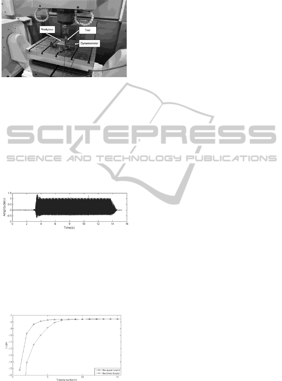
Figure 1: Experimental bench for cutting processing.
The cutting tests were conducted on Mikron
UCP800 Duro, which is a five axis machining centre.
The thrust force was measured by a Kistler 9253823
dynamometer. The resulting signals are converted
into output voltages and then these voltage signals
are amplified by Kistler multichannel charge
amplifier 5070. Force signals were simultaneously
recorded by NI PXIe-1802 data recorder. A 300M
steel work piece material was adopted. The spindle
speed was kept constant at 1000rpm and the feed
rate was 400mm/min. The cutting depth 2mm and
wide 2mm was adopted. A real time cutting signal
with a dull tool processing is shown as Figure 2.
Figure 2: The cutting processing in time domain.
Time domain signals are considered as general
error ±5%, and then the wavelet packet
decomposition is used. The root mean square values
of the wavelet coefficients at different scales were
taken as the feature observations vector. The training
procedure for finding the optimal model is carried
out. The convergence curve of log likelihood is
shown as Figure 3, and hence the convergence of the
GHMM training process can be obtained.
Figure 3: The training convergence curve.
5 CONCLUSIONS
Two kinds of uncertainties in engineering
application can be encountered. The aleraory
uncertainty is derived by the probability measure
while the epistemic uncertainty is modelled by the
generalized interval in GHMM. In this paper, the
generalized convex and concave functions based on
the generalized interval are proposed for inferring
the generalized Jensen inequality. An optimization
method for training GHMM, as a generalization of
Baum-Welch algorithm, is proposed. The
observation sequence is viewed separately as the
lower and the bound observation sequences. The
generalized Baum-Welch’s auxiliary function and
generalized Jensen inequality are used. Similar to
HMM training, a set of training equations has been
derived by optimizing the objective function. The
lower and upper bound re-estimated formulas have
been derived by unique maximum of the objective
function. With a multiple observation concept, a
group of GHMM re-estimation formulas has been
derived. According to multiple observations EM
algorithm, this method guarantees the local
maximum of the lower and upper bound and hence
the convergence of the GHMM training process.
ACKNOWLEDGEMENTS
This research is supported by National Key Basic
Research Program of China (973 Program, Grant
No.2011CB706803), Natural Science Foundation of
China (Grant No. 51175208), and Natural Science
Foundation of China (Grant No. 51075161).
REFERENCES
Jensen, J., L. W. V., 1906. Sur les functions convexes et
les inegalites entre les valeurs moyennes, Acta Math,
30: 175–193.
Rabiner, L. R., 1989. A tutorial on hidden Markov models
and selected applications in speech recognition,
proceedings of the IEEE, 77 (2): 257–286.
Kaucher, E., 1980. Interval analysis in the extended
interval space IR. Computing Supplement, 2:33–49.
Wang, Y., 2011. Multiscale uncertainty quantification
based on a generalized hidden Markov model. ASME
Journal of Mechanical Design, 3: 1–10.
Baum, L. E., Petrie, T, Soules, G., Weiss, Norman., 1970.
A maximization technique occurring in the statistical
analysis of probabilistic functions of Markov chains.
Ann. Math. Statist, 41(1): 164–171.
Li, X. L., Parizeau, M., Plamondon, R., 2000. Training
hidden Markov models with multiple observations – A
An Optimization Method for Training Generalized Hidden Markov Model based on Generalized Jensen Inequality
273

vombinatorial method. IEEE Transactions on PAMI,
(22)4: 371–377.
Popova, E. D., 2000. All about generalized interval
distributive relations. I. Complete Proof of the
Relations Sofia.
Gardenes, E., Sainz, M. A., Jorba, L. Calm, R., Estela, R.,
Mielgo, H., and Trepat, A., 2001. Modal intervals.
Reliable Computing, 2: 77–111.
Markov, S., 1979. Calculus for interval functions of a real
variable Computing, 22(4): 325–337.
Levinson, S., Rabiner, R. and Sondhi. M., 1983. An
introduction to the application of the theory of
probabilistic functions of a Markov process to
automatic speech recognition. Bell Systems Technical
Journal, 62: 1035-1074.
ICINCO 2012 - 9th International Conference on Informatics in Control, Automation and Robotics
274