Flatness based Control of a 2 DOF Single Link Flexible Joint
Manipulator
E. D. Markus
1
, J. T. Agee
1
, A. A. Jimoh
1
, N. Tlale
2
and B. Zafer
3
1
Department of Electrical Engineering, Tshwane University of Technology, Pretoria, South Africa
2
Mobile Intelligent and Autonomous Systems, CSIR, Pretoria, South Africa
3
Department of Mechatronics Engineering, Kocaeli University, Kocaeli, Turkey
Keywords:
Flexible Joint Manipulator, Differential Flatness, Position Control.
Abstract:
The demand for high speed robotic manipulators with little or no vibrations has been a challenging research
problem. In this paper, a position control for a 2 DOF single link flexible manipulator with joint elasticity
is studied. It is shown that using the flatness control approach, faster response and less oscillations and
overshoots can be achieved. The flat output of the linearized system is determined as the tip of the manipulator
end effector. This output and a finite order of its derivatives is defined in terms of the input and states variables
of the manipulator. Using the parameters of the output in flat space, a trajectory is planned and executed to
test the effectiveness of the designed control.
1 INTRODUCTION
The control of flexible robotic manipulators is re-
quired in many applications where faster response,
lower energy consumption, lighter body mass, and
high position accuracy at the end effector are de-
manded. The problem of vibration control in these
systems has been a subject of research over the years
(Ghorbel et al., 1989; Sira-Ramirez et al., 1992;
Ider and
¨
Ozg¨oren, 2000; Ozgoli and Taghirad, 2006;
Tokhi and Azad, 2008; Jiang and Higaki, 2011). Ma-
nipulators with flexible links are difficult to control
due to their slow control response, high oscillations
and high overshoots. The flexible joint manipulator is
also known to exhibit a nonminimum phase behaviour
(Tokhi and Azad, 2008). This makes trajectory track-
ing for the system harder to achieve. From a robot ma-
nipulator design perspective, these disadvantages are
minimised by building the robot from rigid links and
joints that results in high stiffness. However such stiff
systems have been shown to be ineffective in terms of
high power consumption and positional inaccuracy.
Many mathematical and analytical models have
been proposed in the past to achieve control of these
flexible systems (Dwivedy and Eberhard, 2006; Tokhi
and Azad, 2008). Among these include the classical
PID control, feedback linearization, fuzzy logic con-
trol, sliding mode, H∞ control, linear quadratic con-
trol and neuro-fuzzy inference system. A comprehen-
sive survey of research in the control of flexible ma-
nipulators can be found in (Dwivedy and Eberhard,
2006; Ozgoli and Taghirad, 2006).
The concept of differential flatness proposed by
Fliess, Levine, Martin and Rouchon(1995) has been
applied to complex control problems(Fliess et al.,
1995). This study will apply the differential flatness
technique for the control of the single link flexible
joint robot manipulator. The differential flatness ap-
proach through the flat output is used to design an
asymptotically stable controller for suppressing vi-
brations of the flexible joint manipulator. Abdul-
Razak (2007) and Quanser (2012) have reported the
use of the linearized model of the flexible manipu-
lator(Abdul Razak, 2007; Quanser, 2012). The lin-
earized model is simulated with a PID controller and
compared with the flatness based control.
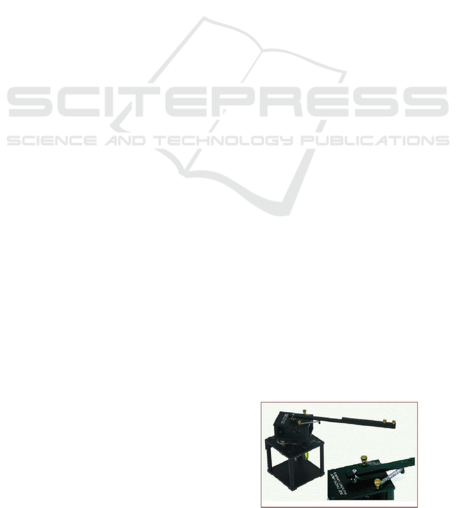
Figure 1: Physical model of flexible joint robot manipulator.
437
D. Markus E., T. Agee J., A. Jimoh A., Tlale N. and Zafer B..
Flatness based Control of a 2 DOF Single Link Flexible Joint Manipulator.
DOI: 10.5220/0004061104370442
In Proceedings of the 2nd International Conference on Simulation and Modeling Methodologies, Technologies and Applications (SIMULTECH-2012),
pages 437-442
ISBN: 978-989-8565-20-4
Copyright
c
 2012 SCITEPRESS (Science and Technology Publications, Lda.)

The main contribution of this study is to show that
using the differential flatness control model, faster re-
sponse and less oscillations and overshoots can be
achieved for the flexible manipulator. Furthermore,
the problem of finding rest to rest trajectories for the
nonminmum phase system is easily achieved without
resorting to iterative solutions by complex numerical
methods.
2 SYSTEM MODELING
The model used for the study is the standard Quanser
flexible joint manipulator platform (Quanser, 2012)
shown in figure(1). The nonlinear dynamic model of
the flexible joint robot is formulated using Lagrange
equations(Groves and Serrani, 2004). Other studies
have used this model to design control for the flexible
manipulator (Abdul Razak, 2007; Akyuz et al., 2011).
However, published results still suffer from oscil-
lations and overshoots due to the flexible nature of
the system. The single link flexible manipulator has a
flexible joint and an arm which is oriented vertically.
This introduces non-linearities in the system as a re-
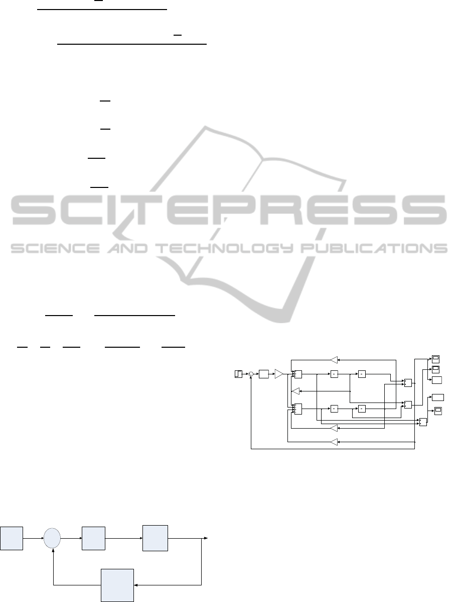
sult of the potential energy due to gravity. Fig (2)
shows the schematic diagram of the single link ma-
nipulator with flexible joint.
The input to the system is the voltage applied to
the motor and the output is the tip angle which is
a sum of the motor angle and the joint deflection .
The system has two degrees of freedom which corre-
sponds to the motor rotation angle and the rotation of
the flexible joint . The coordinates of the flexible joint
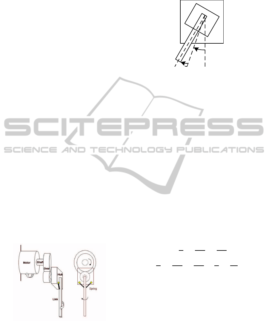
manipulator are reflected in fig(3).
Figure 2: The schematic diagram of single link flexible ma-
nipulator with flexible joint.
Removing the nonlinear sinusoids enables the
computation of the flat output for the linear system.
This is computed using the technique proposed by
(Levine and Nguyen, 2003). The energy equation for
the system is formulated using the Lagrangian energy
θ
α
Figure 3: Co-ordinates of the flexible joint manipulator.
equation.
L = K −V (1)
where
K = K
h
+ K
l
V = V
g
+V
s
(2)
K and V are kinetic and potential energy respec-
tively. For a complete derivation of the dynamic
model of the single link flexible joint manipulator,see
(Akyuz et al., 2011). Choosing our state variables as:
θ = x
1
˙
θ = x
2
α = x
3
˙
α = x
4
(3)
The linearized equations of motion about zero
equilibrium point of the manipulator represented in
state space are given as a fourth order system in the
equation below:
˙
x =





x
2
K
s
J
h
x
3
−
K
2
m
K
2
g
R
m
J
h
x
2
+
K
m
K
g
R
m
J
h
V
x
4
−
K
s
J
h
x
3
+
K
2
m
K
2
g
R
m
J
h
x
2
−
K
m
K
g
R
m
J
h
V −
K
s
J
l
x
3
+
mgh
J
l
(x
1
+ x
3
)





(4)
2.1 Differential Flatness
A linear system
f(x, ˙x, u)
x ∈ ℜ
n
, u ∈ ℜ
m
, n ≥ m+ 1 (5)
is said to be differentially flat if there exists a variable
or set of variables h
1
∈ ℜ
n
called the flat output of the
form:
h
1
= y(x, u, ˙u, ¨u, ......, u
(p)
) (6)
defined by:
SIMULTECH2012-2ndInternationalConferenceonSimulationandModelingMethodologies,Technologiesand
Applications
438

x = α(h
1
,
.
h
1
,
.
h
1
, ......, h
1
(q)
),
u = β(h
1
,
.
h
1
,
.
h
1
, ......, h
1
(q+1)
) (7)
p and q are finite integers, Such that the system of
equations
d
dt
α(h
1
,
.
h
1
,
.
h
1
, ......, h
1
(q+1)
) =
f(α(h
1
,
.
h
1
,
.
h
1
, ......, h
1
(q)
), β(h
1
,
.
h
1
,
.
h
1
, ......, h
1
(q+1)
))
(8)
are identically satisfied (Rouchon et al., 1993).
2.2 Determination of the Flat Output
According to Levine and Nguyen (2003), a linear
system of the form of equation (4) with one input
can be expressed in terms of equation (9)(Levine and
Nguyen, 2003).
A(s)x = Bu (9)
where x = P(s)h
1
(s), u = Q(s)h
1
(s) and A(s) = sI−A
The variable h
1
= (h
1
........h
m
) is the linear flat
output and the matrices P and Q are given by equa-
tions (10) and (11) respectively
C
T
A(s)P(s) = 0 (10)
A(s)P(s) = BQ(s) (11)
The matrix C is an n× (n− m) matrix of rank n-m
orthogonal to B such that:
C
T
B = 0 (12)
and
Q(s) = (B
T
B)
−1
B
T
A(s)P(s) (13)
Expressing equation (4) in terms of A(s), we have
A(s) =





0 −1 0 0
0 s+
K
2
m
K
2
g
R
m
J
h
−
K
s
J
h
1
0 0 s −1
−
mgh
J
l
−
K
2
m
K
2
g
R
m
J
h
K
s
J
h
+
K
s
J
l
−
mgh
J
l
s





(14)
B
T
=
h
0
K
m
K
g
R
m
J
h
0 −
K
m
K
g
R
m
J
h
i
(15)
For C
T
B = 0 we select
C
T
=


1 0 0 0
0 1 0 1
0 0 1 0


(16)
Noting that
P(s) =

P
1
(s) P
2
(s) P
3
(s) P
4
(s)

(17)
Equation (10) will yield
P
1
(s) =

s
2
+
K
s
− mgh
J
l

h
1
(s)
P
2
(s) = sP
1
(s)
P
3
(s) =

−s
2
+
mgh
J
l

h
1
(s)
P
4
(s) = sP
3
(s) (18)
From equation (18), we can express all the states
of the system in terms of the flat output h
1
and its
derivatives
x
1
(t) = θ(t) =
..
h
1
(t) +
K
s
− mgh
J
l
h
1
(t)
x
2
(t) =
.
θ
(t) =
...
h
1
(t) +
K
s
− mgh
J
l
.
h
1
(t)
x
3
(t) = α(t) = −
..
h
1
(t) +
mgh
J
l
h
1
(t)
x
4
(t) =
.
α
(t) = −
...
h
1
(t) +
mgh
J
l
.
h
1
(t) (19)
and u(t) = v
From equation (13), Q(s) = (B
T
B)
−1
B
T
A(s)P(s)
yields
Q(s) = β
1
s
4
+ β
2
s
3
+ β
3
s
2
+ β
4
s+ β
5
(20)
where:
β
1
=
J
h
R
m
K
g
K
m
β
2
= K
g
K
m
β
3
=
K
s
R
m
2K
g
K
m
+ J
h
R
m
(
K
s
J
h
+
K
s
J
l
−
mgh
J
l
)
2K
g
K
m
+
J
h
R
m
(K
s
− mgh)
2K
g
K
m
J
l
β
4
=
K
g
K
m
(K
s
− mgh)
J
l
and
β
5
=
mghR
m
J
h
(K
s
− mgh)
2K
g
K
m
J
l
2
−mgh
K
s
R
m
+ J
h
R
m
(
K
s
J
h
+
K
s
J
l
−
mgh
J
l
)
2K
g
K
m
J
l
Putting
K
s
−mgh
J
l
= W and
mgh
J
l
= Y into equation (20)
Then u(t) becomes
u(t) =
J
h
R
m
K
g
K
m
h
1
(4)
+ K
g
K
m
h
1
(3)
FlatnessbasedControlofa2DOFSingleLinkFlexibleJointManipulator
439

+[
K
s
R
m
+ J
h
R
m
(
K
s
J
h
+W) + J
h
R
m
W
2K
g
K
m
]
..
h
1
+K
g
K
m
W
.
h
1
+
R
m
J
h
YW −YK
s
R
m
− R
m
J
h
Y(
K
s
J
h
+W)
2K
g
K
m
h
1
(21)
Expressing the flat output h1 in terms of the states
h
1
(t) =
J
l
K
s
(θ+ α)
˙
h
1
(t) =
J
l
K
s
(
.
θ
+
.
α
)
¨
h
1
(t) =
mgh
K
s
(θ+ α) − α
h
(3)
1
(t) =
mgh
K
s
(
.
θ
+
.
α
) −
.
α
(22)
A new states space model in terms of the flat out-
put variables called the Brunovskys model can now
be described for the original manipulator system as:
˙
h
1
= h
2
˙
h
2
= h
3
˙
h
3
= h
4
˙
h
4
=
mghK
s
J
l
J
h
h
1
−
(K
g
K
m
)
2
(K
s
− mgh)
J
l
J
h
R
m
h
2
−[
K
s
J
h
+
K
s
J
l
−
mgh
J
l
]h
3
−
(K
g
K
m
)
2
J
h
R
m
h
4
+
K
g
K
m
J
h
R
m
u(t)
(23)
3 CONTROLLER DESIGN
Designing the controller in flat output space is easy
since the manipulator is represented by a chain of in-
tegrators. The flatness property decouples dynamics
of the position, velocity, acceleration and jerk. Their
trajectories can easily be generated without differenti-
ation. It should be noted that only the tip position was
used for feedback. Figure (4) illustrates the block di-
agram of the flatness based control.
Feedback
Controller
∑
Flexible
Manipulator
Transformation
to flat
coordinates
Reference
Trajectory
e
u
y
h1
+
-
Figure 4: Block diagram of flatness based control for the
flexible joint robot manipulator.
The reference trajectory is generated from the end
effectortip position which is the flat output of the flex-
ible manipulator. The state variables are transformed
to flat output coordinates. The aim of the control is
to track the position of the end effector as precisely
as possible. Based on the linear system of equation
(23), a controller will now be designed using the flat
variables. For the 4th order system:
˙
h
4
(t) =
ˆ
h
4d
− K
1
(h
1
(t) −
ˆ
h
1d
(t)) − K
2
(h
2
(t) −
ˆ
h
2d
(t))
−K
3
(h
3
(t) −
ˆ
h
3d
(t)) − K
4
(h
4
(t) −
ˆ
h
4d
(t)) (24)
This can be written in the form
.
h
4
(t) =
ˆ
h
4d
− K
1
e− K
2
.
e
−K
3
..
e
−K
4
...
e
(25)
where
e = h
1
−
ˆ
h
1d
,
.
e
= h
2
−
ˆ
h
2d
,
..
e
= h
3
−
ˆ
h
3d
,
...
e
=
h
4
−
ˆ
h
4d
K
i
, i = 1, 2, 3, 4 are the controller gains.
The expression in the complex field is
s
4
+ K
4
s
3
+ K
3
s
2
+ K
2
s+ K
1
= 0 (26)
The K parameters have to be chosen to minimise
the system error. PID is used to tune the gains
and drive the system error to a minimum. Figure
(5) shows the simulation environment for the linear
model in Simulink.
x1_d t
x1
x3
x3_d tdt
x3_d t
x1_d tdt
vel
positi on
accn
simou t4
To Workspace1
simou t6
To Workspace
Step
PID(s)
PID Con troller
1
s
Inte grato r3
1
s
Inte grato r2
1
s
Inte grato r1
1
s
Inte grato r
-K-
Gai n5
-K-
Gai n3
-K-
Gai n2
-K-
Gai n1
-K-
Gai n
Add 4
Add 3
Add 2
Add 1
Add
Figure 5: Simulink diagram of the linear model.
4 SIMULATION AND RESULTS
It is required to generate smooth point to point end
effector tip movements. For position control, motion
that has a velocity of zero at the start of motion and at
the end is desired. The motion should also accelerate
and decelerate smoothly. To check for the control-
lability of the modelled flexible manipulator, time re-
sponse analysis was carried out. Results show that the
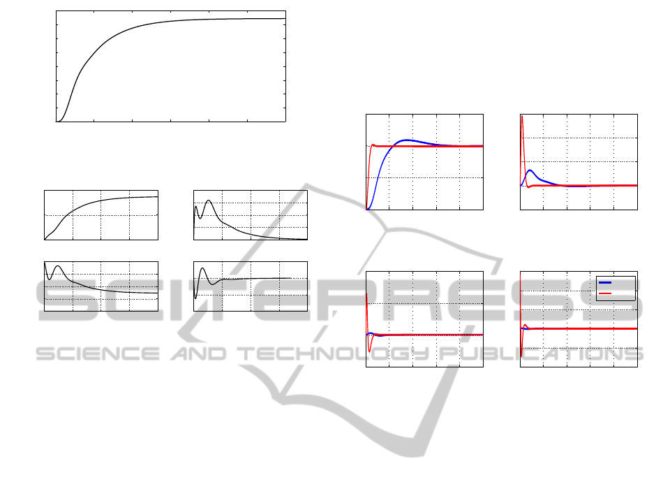
system is stable and controllable. Figure (6) shows
the response of the tip position (θ+α) to a step input.
SIMULTECH2012-2ndInternationalConferenceonSimulationandModelingMethodologies,Technologiesand
Applications
440

0 0.5 1 1.5 2 2.5 3
0
0.1
0.2
0.3
0.4
0.5
0.6
0.7
0.8
Time (secs)
theta+alpha(rads)
Tip displacement
Figure 6: Step response of end effector position (θ + α)
based on linear model.
0 0.5 1 1.5 2
0
0.5
1
Time (s)
Theta(rads)
0 0.5 1 1.5 2
0
0.5
1
1.5
2
Time(s)
theta vel.(rads/s)
0 0.5 1 1.5 2
−0.2
−0.15
−0.1
−0.05
0
Time(s)
alpha(rads)
0 0.5 1 1.5 2
−2
−1
0
1
Time(s)
alpha vel.(rads/s)
Figure 7: Step responses of motor angle (θ), joint displace-
ment (α) and their velocities.
The step input introduces an instantaneous rota-
tion on the motor shaft and results in a joint deflec-
tion. The system has a rise time of 0.84s, a settling
time of 1.6s and steady state of 0.74rads with no over-
shoots. This response is satisfactory given that the
flexible manipulator model has been linearized. A
further check on the motor angle response and joint
deflection and their velocities gives an insight of a sta-
ble system. The plots of figure (7) show the time re-
sponse on motor angle θ and joint deflection α of the
linear flexible manipulator model.
In order to check the steady sate error performance
of the proposed control, a closed loop feedback con-
trol was carried out as shown in figure (4). Compar-
isons were made from simulation results obtained for
two different controlled platforms of the flexible ma-
nipulator using the MATLAB/Simulink environment.
Position control is carried out on the linearized model
and then compared with the flatness based model.
The results in figure (8) shows that both PID
control and the flatness based control, achieved zero
steady state error. The flatness based control has a
percentage overshoot of less than 2% while the PID
control has 9%. This is caused by the instantaneous
effect of the step input on the motor. This effect can
be seen by the large overshoots in the velocity and
jerk. The reference trajectory however quickly settles
to steady state with a settling time of 1.8s for the lin-
ear PID control. When compared to the flatness based
control, a faster settling time of 0.3s is observed. This
means that the flatness based control is more toler-
ant to oscillations and vibrations much more than the
classical PID control. An observation of nonmini-
mum phase behaviour was made in the linear flat dy-
namics. The plots in figure (8) show that the Flatness
based controller was able to resolve this problem.
0 0.5 1 1.5 2 2.5
0
0.5
1
1.5
Tip displacement
h1(rads)
0 0.5 1 1.5 2 2.5
−5
0
5
10
15
Tip velocity
Velocity(rads/s)
0 0.5 1 1.5 2 2.5
−500
0
500
1000
acceleration
accn(rads/s
2
)
Time(s)
0 0.5 1 1.5 2 2.5
−4
−2
0
2
4
6
x 10
4
Jerk
jerk(rads/s
3
)
Time(s)
PID Control
Flat Control
Figure 8: Comparison of system response based on PID and
flatness based control.
5 CONCLUSIONS
This paper has presented a control for a single link
flexible joint robot manipulator. The flat output for
a linearized model of the manipulator was derived.
The model was analysed and control designed based
on differential flatness. The PID control on the lin-
ear model was compared with control of the flat-
ness based model. Results show a satisfactory perfor-
mance on the dynamics and control of both platforms.
The flatness based control however shows faster re-
sponse to instantaneous motor displacement with lit-
tle vibrations and less overshoots.
REFERENCES
Akyuz, I. H., Yolacan, E., Ertunc, H. M., and Bingul, Z.
(2011). Pid and state feedback control of a single-
link flexible joint robot manipulator. In Mechatronics,
pages 409–414. IEEE.
Dwivedy, S. and Eberhard, P. (2006). Dynamic analysis of
flexible manipulators, a literature review. Mechanism
and Machine Theory, 41(7):749–777.
Fliess, M., Lvine, J., Martin, P., and Rouchon, P. (1995).
Flatness and defect of non-linear systems: introduc-
FlatnessbasedControlofa2DOFSingleLinkFlexibleJointManipulator
441

tory theory and examples. International journal of
control, 61(6):1327–1361.
Ghorbel, F., Hung, J., and Spong, M. (1989). Adaptive con-
trol of flexible-joint manipulators. Control Systems
Magazine, IEEE, 9(7):9–13.
Groves, K. and Serrani, A. (2004). Modeling and nonlinear
control of a single-link flexible joint manipulator.
Ider, S. K. and
¨
Ozg¨oren, M. K. (2000). Trajectory tracking
control of flexible-joint robots. Computers & Struc-
tures, 76(6):757–763.
Jiang, Z. H. and Higaki, S. (2011). Control of flexible joint
robot manipulators using a combined controller with
neural network and linear regulator. Proceedings of
the Institution of Mechanical Engineers, Part I: Jour-
nal of Systems and Control Engineering, 225(6):798–
806.
Lvine, J. and Nguyen, D. V. (2003). Flat output character-
ization for linear systems using polynomial matrices*
1. Systems & control letters, 48(1):69–75.
Ozgoli, S. and Taghirad, H. D. (2006). A survey on the con-
trol of flexible joint robots. Asian Journal of Control,
8(4):332–344.
Quanser (2012).
Razak, N. B. A. (2007). Modelling of single link flexible
manipulator with flexible joint. PhD thesis, Universiti
Teknologi Malaysia.
Rouchon, P., Fliess, M., Lvine, J., and Martin, P. (1993).
Flatness, motion planning and trailer systems. In Proc.
Conf. on Decision and Control, pages 2700–2705 vol.
3. IEEE.
Sira-Ramirez, H., Ahmad, S., and Zribi, M. (1992). Dy-
namical feedback control of robotic manipulators with
joint flexibility. Systems, Man and Cybernetics, IEEE
Transactions on, 22(4):736–747.
Tokhi, M. O. and Azad, A. K. M. (2008). Flexible robot
manipulators: modelling, simulation and control, vol-
ume 68. London Institution of Engineering and Tech-
nology.
SIMULTECH2012-2ndInternationalConferenceonSimulationandModelingMethodologies,Technologiesand
Applications
442