Estimating Real Process Derivatives in on-Line Optimization

A Review

M. Mansour

Faculty of Electronics and Computer Science, USTHB, PO. BOX 32, El_Allia. Bab-Ezzouar, Algiers, Algeria

Keywords: on-Line Optimization, Model-based, Process Derivatives, ISOPE Algorithm, ANN.

Abstract: The solution of the Integrated System Optimization and Parameter Estimation (ISOPE) problem necessitates

the calculus of real process output derivatives with respect to the inputs. This information is needed in order

to satisfy first and second order optimality conditions. Several methods exist and have been developed for

calculating these derivatives. In this paper a review of most of the existing methods is presented, in which

the Finite Difference Approximation, Dual Control Optimization, Broydon’s method, Dynamic Model

Identification, with both linear and nonlinear models, together with a neural networks scheme are presented

and applied, under simulation, to a cascade Continuous Stirred Tank Reactor (CSTR) system. The results

are then discussed and compared to identify the advantages and disadvantages of using each method.

1 INTRODUCTION

The requirement for processes to operate at their

optimum operating condition is becoming

increasingly prevalent. One model-based algorithm

that has been developed and which can achieve

optimum process operation in spite of model-reality

mismatch is the Integrated System Optimization and

Parameter Estimation (ISOPE) algorithm (Roberts,

1979). One requirement of the ISOPE algorithm, in

order to satisfy the necessary optimality conditions,

is the need for estimates of real process derivatives.

These derivatives are estimated on-line at each

iteration of the algorithm. The finite difference

method originally used by Roberts (1979) to

estimate these derivatives has proven not to be

efficient in the case of large, slow and noisy

processes (Mansour and Ellis, 2003). Alternative

methods have therefore been developed. The

dynamic model identification technique, which is

based on the identification of a dynamic model, was

incorporated within the ISOPE algorithm by Zhang

and Roberts (1990). Although this technique proved

to be fast enough as it performs the identification

during transient, it encountered some difficulties

such as: the huge amount of data needed and the

poor, inaccurate, model it produces at the beginning

of the identification. After that, an algorithm with

dual control effect was proposed (Brdys and

Tatjewski, 1992). In this algorithm the current

control signal is generated to satisfy the main control

goal and at the same time provide sufficient

information for future identification action. The

main advantage of this algorithm is that it does not

need excessive set-point changes to estimate the

process derivatives. However, this method

encountered the same type of problems as the

previous ones. Broydon's approximation method

based on the well-known Broydon’s family of

formulas which are mainly oriented to the

approximation of derivatives was also implemented

(Fletcher, 1980). Lately, a nonlinear version of the

dynamic model identification was applied and

implemented (Mansour and Ellis, 2003). In this

paper, a review of all these techniques together with

a method based on artificial neural networks is

presented. In addition, a comparison is made using

simulations carried out on a cascade CSTR system

to show the advantages and disadvantages of each

method.

2 THE OPTIMIZATION

PROBLEM AND THE ISOPE

ALGORITHM

We The ISOPE algorithm (or modified two steps)

was proposed by Roberts (Roberts, 1979) to solve

the general optimization problem of finding the

120

Mansour M..

Estimating Real Process Derivatives in on-Line Optimization - A Review.

DOI: 10.5220/0004059101200124

In Proceedings of the 2nd International Conference on Simulation and Modeling Methodologies, Technologies and Applications (SIMULTECH-2012),

pages 120-124

ISBN: 978-989-8565-20-4

 2012 SCITEPRESS (Science and Technology Publications, Lda.)

optimum operating point of a system while it is

moving from one operating point to another. It uses

an adaptive steady-state model of the process, in

which the parameters are updated periodically by

comparing model outputs with those of the real

process.

The general form of the algorithm is given as

follows (Mansour and Ellis, 2008):

Apply the current input

to the real process and

wait for the system to settle down to obtain steady-

state measurement

. Then use the existing

mathematical model to determine the model

parameters

to minimize the comparison index

given by:

(, )

()

()0

Min Gu

≤

(1)

where

(, ) ,(())

ii i

Gu w y h u

αα

= −

∑

%%%%

(2)

and

is a weighting vector.

Solve the modified model-based optimization

problem given by:

((, (,)) )

()

()0

Min Q Huu u

yHv

−

≤

%% %

(3)

In order to obtain the new candidate

Where

yy yQ

−

⎡⎤

∂∂ ∂∂

⎡⎤ ⎡⎤⎡⎤

⎢⎥

=−

⎢⎥

⎢⎥ ⎢⎥⎢⎥

∂∂∂∂

⎣⎦ ⎣⎦⎣⎦

⎢⎥

⎣⎦

%% %

(4)

λ is called a modifier and is obtained following

consideration that the necessary optimality

conditions, of the system optimization problem,

have to be satisfied (Roberts, 1979; Ellis et al., 1988;

Roberts and Williams, 1981).

However, the new control

is not directly

applied to the system for stability reasons. Instead,

the following relaxation scheme is used:

=+( )

kk kk

vvKuv

−

%% %%

(5)

where K is a relaxation gain matrix and is a tuning

parameter.

These steps are repeated until convergence is

reached. Convergence occurs when no further

improvement is observed. In other words, when the

new control is no longer a better candidate than the

previous one and the objective function has reached

its minimum within the possible bounds determined

by the equality and inequality constraints

However, and from the previous cited relations, it

can be seen that the requirement of the ISOPE

algorithm to measure real process output

derivatives with respect to the set-points

⎡⎤

∂∂

⎣⎦

compute the modifier λ imposes a practical

limitation to the technique. These process

derivatives are calculated online, usually by

applying small perturbations on the set-points and

measure the resulting changes on the outputs. This

process is repeated at each iteration of the algorithm.

Various techniques exist and have been developed

and applied for the purpose of estimating these

derivatives. The Finite differences technique was

originally suggested with the modified two step

method (Roberts, 1979). Dynamic Model

Identification (DMI) using a linear model was then

applied by Zhang and Roberts (1990). An algorithm

for dual control effect was also suggested and

implemented (Brdys and Tatjewski, 1992). Also, a

method based on the well known Broydon Formula

was proposed and tested (Fletcher, 1980). Lately,

DMI with a nonlinear model was proposed and

implemented on a two CSTR system

(Mansour and

Ellis, 2003). In this work, a method based on

Artificial Neural Networks (ANN) to estimate the

real process derivatives and predict future control

actions is presented. In this method, a static neural

network model of the real system is created, trained

and adapted to the behavior of the system. This

model, imitates the behavior of the real system

within its limits. The aim is to use this steady-state

model to estimate the real system output derivatives

with respect to the set-points in order to compute the

parameter λ. All the above techniques are

implemented and tested under simulation on a two

CSTR system.

3 SIMULATIONS AND RESULTS

In order to assess and compare the performances of

the techniques mentioned above, a set of simulations

were carried out on a two Continuous Stirred Tank

Reactors (CSTR) connected in cascade (Garcia and

Morari, 1981). An exothermic autocatalytic reaction

takes place in the reactors with interaction taking

EstimatingRealProcessDerivativesinon-LineOptimization-AReview

121

place in both directions due to a recycle of 50% of

the product stream into the first reactor.

The reaction is:

−

+⇔

(6)

The manipulated variables which are the set-points

of the temperature controllers in both reactors are:

(, )

vTT=

. The product concentrations associated

with the second tank are outputs:

(,)

yCaCb=

The objective function for all the simulations using

this system was chosen to be linear of the measured

variable and reflects the desire of maximizing the

amount of component B in tank 2. Thus the form of

the objective function is as follow:

(,)

yv C

−

(7)

The simulations were carried out using a

MATLAB

/ Simulink platform. The starting point

which is the initial steady-state condition was

chosen to be: T

(0)=307 K and T

(0)=302 K which

yields the following steady -state outputs:

=0.0141[kmol/m

] and Cb

=0.0586[kmol/m

In the simulations, the identification of the

dynamic model within the DMI method (with linear

or non-linear model) was carried out during

transient, once found the updated model was used in

the model-based optimization routine to produce the

new process set-points. The identifier parameters

were chosen as given in Table 1.

Table 1: Tuning the identifier parameters.

Linear Model

Non-linear

Model

Length of data

window

= 120 N

= 60

Model

orders

= 2, n

= 5,

=1, d = 1

d = 1

Identifier

sampling time

= 60s T

= 60s

Relaxation gain K = 0.03I K = 0.1I

For the neural network scheme, a feedforward back-

propagation neural network composed of eight input

neurons, five hidden layers and two output neurons

was used in the simulation. In a feedforward

network, the first layer has weights coming from the

input. Each subsequent layer has a weight coming

from the previous layer. The last layer is the network

output.

It has to be mentioned that the choice of the

number of layers and their neurons depend totally on

the experimenter. The main factor to be taken into

account is the algorithm behaviour towards the

different values tested. In practice, the algorithm

can be tested with different combinations of layers

in simulations based on robust models of the system.

The optimum (best) choice is then applied on the

real system.

The final converged results of the simulations for

the various techniques are shown in Table 2 and

figures 1 to 6.

Table 2 gives the final objective function value

and the number of set-point changes taken to

converge to the optimum point, obtained using all

the techniques presented in this paper. While the

figures show the trajectories taken by the outputs

and manipulated variables.

We notice that all the methods converge to the

correct process optimum point given by

T =312 K

and

T =310.2K

, with the optimum objective

function value of -0.0725. From Figures 1 to 6, it is

seen how the changes in the set-points affect the

measured outputs and how they derive their values

from the initial steady-state condition given by

(0)=0.041361 [kmol/m

], Cb

(0)=0.058638

[kmol/m

] to the final desired solution (Ca

=0.0275

[kmol/m

], Cb

=0.0725 [kmol/m

]).

Table 2: ISOPE algorithm with the different estimation

techniques.

Objective

function value

Number of set-

point changes

FDAM -0.0725 22

Broydon’s

method

-0.0725 12

Dual control

method

-0.0725 14

DMI with linear

model

-0.0725 12

DMI with non-

linear model

-0.0725 10

Neural network

method

-0.0725 7

Figure 1: FDAM method.

0 0.5 1 1.5 2

x 10

0.02

0.04

0.06

Ca2 (kmol/m3)

Time (s)

0 0.5 1 1.5 2

x 10

0.04

0.06

0.08

Cb2 (kmol/m3)

Time (s)

0 0.5 1 1.5 2

x 10

300

305

310

315

T1 (K)

Time (s)

0 0.5 1 1.5 2

x 10

300

305

310

315

T2 (K)

Time (s)

SIMULTECH2012-2ndInternationalConferenceonSimulationandModelingMethodologies,Technologiesand

Applications

122

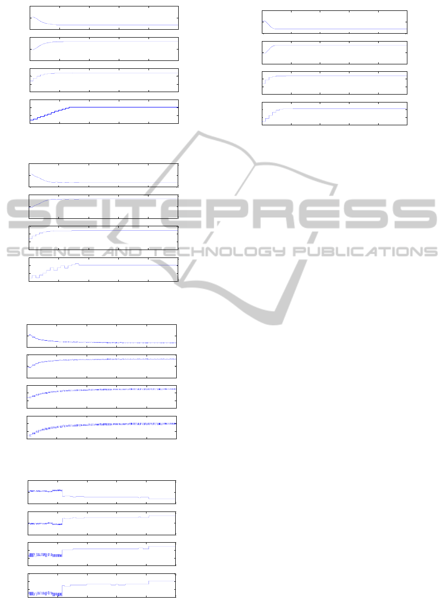
Figure 2: Broydon’s method.

Figure 3: Dual control method.

Figure 4: DMI with a linear model.

Figure 5: DMI with a nonlinear model.

Figure 6: The Neural network method.

4 DISCUSSION AND

CONCLUSIONS

Techniques for estimating real process derivatives to

be used within the ISOPE algorithm have been

reviewed, and applied on a cascade process

consisting of two Continuous Stirred Tank Reactors.

All methods, due to the satisfaction of optimality

conditions, do achieve the real process optimum

provided they can be implemented in a stable

manner after a suitable choice of relaxation gains.

In the case of high order, slow and noisy

processes, the FDAM, is not, as is well documented,

a good choice. Each time a process derivative is

requested, a set-point perturbation needs to be

applied and a measurement time needs to be given to

allow the process to settle before the derivatives are

measured. Additional difficulties are observed when

noise is present on the output measurement. This set-

point perturbation, and the subsequent measurement

time, is where the majority of time is spent in the

algorithm so this is a major consideration in

assessing the algorithm. As can be seen from the

simulation results on the CSTR’s system (Table 2),

the FDAM, approaches twice the number of set-

point changes of the various after methods and

would seem not to be the perfect choice of

algorithm.

The dual control method takes 14 set-point

changes (Table 2) to achieve the optimum in the

CSTR’s simulation. This is still more than the after

methods but the ability of the algorithm to estimate

the derivatives without any excess in the set-point

changes makes it a good choice. It has to be

mentioned that the ISOPE using the dynamic model

identification with a nonlinear model gives better

results than that using a linear one. This is

demonstrated by the number of set-point changes

0 2 4 6 8 10

x 10

0.02

0.04

0.06

Ca2 (kmol/m3)

Time (s)

0 2 4 6 8 10

x 10

0.04

0.06

0.08

Cb2 (kmol/m3)

Time (s)

0 2 4 6 8 10

x 10

300

305

310

315

T1 (K)

Time (s)

0 2 4 6 8 10

x 10

300

305

310

315

T2 (K)

Time (s)

0 2 4 6 8 10

x 10

0.02

0.04

0.06

Ca2 (kmol/m3)

Time (s)

0 2 4 6 8 10

x 10

0.04

0.06

0.08

Cb2 (kmol/m3)

Time (s)

0 2 4 6 8 10

x 10

300

305

310

315

T1 (K)

Time (s)

0 2 4 6 8 10

x 10

300

305

310

315

T2 (K)

Time (s)

0 2 4 6 8 10

x 10

0.02

0.04

0.06

Ca2 (kmol/m3)

Time (s)

0 2 4 6 8 10

x 10

0.04

0.06

0.08

Cb2 (kmol/m3)

Time (s)

0 2 4 6 8 10

x 10

300

305

310

315

T1 (K)

Time (s)

0 2 4 6 8 10

x 10

300

305

310

315

T2 (K)

Time (s)

0 2 4 6 8 10

x 10

0.02

0.04

0.06

Ca2 (kmol/m3)

Time (s)

0 2 4 6 8 10

x 10

0.04

0.06

0.08

Cb2 (kmol/m3)

Time (s)

0 2 4 6 8 10

x 10

300

305

310

315

T1 (K)

Time (s)

0 2 4 6 8 10

x 10

300

305

310

315

T2 (K)

Time (s)

0 2 4 6 8 10

x 10

0.02

0.04

0.06

Ca2 (kmol/m3)

Time (s)

0 2 4 6 8 10

x 10

0.04

0.06

0.08

Cb2 (kmol/m3)

Time (s)

0 2 4 6 8 10

x 10

300

305

310

315

T1 (K)

Time (s)

0 2 4 6 8 10

x 10

300

305

310

315

T2 (K)

Time (s)

EstimatingRealProcessDerivativesinon-LineOptimization-AReview

123

taken to reach the optimum point which is fewer in

the first method. In this paper and using the CSTR

example, the most suitable method is the neural

network scheme as only 07 set-point changes are

needed in order to converge to the right optimum

point. However, the huge amount of data needed for

training the network is its major drawback.

REFERENCES

Brdys, M. A. and Tatjewski, P., 1994. An algorithm for

steady-state optimizing dual control of uncertain

plants, paper presented at the 1

IFAC Workshop on

new trends in design of control systems, September 7 -

10, Smolenice, Slovak Republic, pp 249-254.

Ellis, J. E., Kambhampati, C., Sheng, G. and Roberts,

P.D., 1988. Approaches to the optimizing control

problem, Int. J. of Systems Science, Vol. 19, No. 10,

pp 1969-1985.

Fletcher, R., 1980. Practical Methods of Optimization,

Vol.1, A. Wiley-Interscience Publication.

Garcia, C. E. and Morari, M., 1981. Optimal operation of

integrated processing Systems, AICHE Journal, Vol.

27, No. 6, pp 960-968.

Mansour, M. and Ellis, J. E., 2003. Comparison of

methods for estimating real process derivatives in on-

line optimisation, Applied Mathematical Modeling,

Vol. 27, pp 275-291.

Mansour, M. and Ellis, J. E., 2008. Methodology of on-

line optimization applied to a chemical process,

Applied Mathematical Modeling, Vol. 32, pp 170-184.

Roberts, P. D., 1979. An algorithm for steady-state system

optimization and parameter estimation, Int. J. of

Systems Science, Vol. 10, pp 719-734.

Roberts, P. D, and Williams. T. W. C., 1981. On an

algorithm for combined system optimisation and

parameter estimation, Automatica, Vol. 17, pp 199-

209.

Zhang, H. and Roberts, P.D., 1990. On-line steady-state

optimisation of nonlinear constrained processes with

slow dynamics, Trans Ins MC, Vol. 12, No 5, pp 251-

261.

SIMULTECH2012-2ndInternationalConferenceonSimulationandModelingMethodologies,Technologiesand

Applications

124