
Success Probability Evaluation of Quantum Circuits
based on Probabilistic CNOT-Gates
Amor Gueddana, Rihab Chatta and Noureddine Boudriga
Communication Network and Reserach Laboratory (CNAS), Engineering School of Communication of Tunis (SUP’COM),
Ghazala Technopark, 2083, Ariana, Tunisia
Keywords:
CNOT, C
k
NOT, Abstract Probabilistic CNOT, Quantum CNOT-based Circuit.
Abstract:
In this paper, we study the effect of non deterministic CNOT gates on the success probability of Quantum
CNOT-based circuits. Based on physical implementation, we define an abstract probabilistic model of the
CNOT gate that takes into consideration error sources and realizability constraints. Using the proposed model,
we simulate a three-qubit quantum adder and show the evolution of the probability of realizing correctly the
SUM operation depending on the success probability and errors of the CNOT gates.
1 INTRODUCTION
Controlled-NOT gates associated with single qubits
operation are universal for building quantum circuits
(Nakahara and Ohmi, 2008). Quantum CNOT gates
based on linear optics still presents some conceptual
and realization problems. It has been shown that the
use of linear components doesn’t permit to reach de-
terministic gates. Several works proposed non deter-
ministic CNOT gate functioning at least with a suc-
cess probability of 1/4. Some of these gates were
physically realized and the expected result is quite
consistent with theoretical modeling, this is due es-
sentially to unexpected errors caused by the imper-
fection of linear components. We believe that stud-
ies concerning errors affecting the functioning of the
CNOT gate is missing modeling.
Quantum circuits based on CNOT gates were sim-
ply treated in the ideal case where the gate works per-
fectly. All what has been said about the use of non de-
terministic gates is that the success probability of re-
alizing a function will exponentially decrease depend-
ing on the number of gates used. To our knowledge,
no detailed study were achieved to show the behavior
of quantum circuit against non deterministic gates.
Our contribution in this work is three fold: first,
we propose an error control model of an abstract
probabilistic CNOT gate, while taking into consider-
ation physical implementation constraints. Second,
we identify errors affecting the success probability of
the gate at the implementation level and we model
errors related to the basic quantum linear compo-
nents. Third, based on physical implementation of
the TC.Ralph CNOT model, we define a set ofCNOT
gates having the form of an abstract CNOTgate that
are physically realizable and extend our results to the
probabilistic algorithms.
This paper is organized around five sections. Sec-
tion 2 introduces the universality of CNOT gates and
illustrates briefly several steps used to get CNOT de-
composition of C
k
NOT gate. In section 3, we present
first a model of an abstract probabilistic CNOT gate
and based on the TC.Ralph model, a subspace of re-
alizable probabilistic gate is presented, second, we
study the errors caused by linear components and
model their effect at the implementation level. Sec-
tion 4 presents in a first hand, a scheme for model-
ing probabilistic CNOT-based quantum circuits and
in a second hand, the CNOT based three qubit Min-
imized Quantum Ripple Carry Adder is treated as a
case study. Finally some numerical experimentation
are illustrated.
2 QUANTUM CNOT-BASED
CIRCUITS
2.1 Quantum C
k
NOT Gate
In the general form, a single qubit quantum gate has a
unitary 2×2 matrix representation denoted by u and
having the following expression:
378
Gueddana A., Chatta R. and Boudriga N..
Success Probability Evaluation of Quantum Circuits based on Probabilistic CNOT-Gates.
DOI: 10.5220/0004058503780387
In Proceedings of the International Conference on Data Communication Networking, e-Business and Optical Communication Systems (OPTICS-2012),
pages 378-387
ISBN: 978-989-8565-23-5
Copyright
c
2012 SCITEPRESS (Science and Technology Publications, Lda.)

u =
u
00
u
01
u
10
u
11
(1)
where u
00
, u
01
, u
10
and u
11
∈C and describing the
amplitude probability of being in a specific quantum
state (Figure 1a).
Figure 1: General form of a quantum gate.
We consider two major single qubit operations for
building quantum circuits:
I
2
= |0ih0|+ |1ih1| =
1 0
0 1
(2)
U
NOT
= |1ih0|+ |0ih1| =
0 1
1 0
(3)
A C
k
u gate, where k ∈ N
∗
+
, is a gate acting on
(k+ 1) qubits. It inverts the state of the last qubit if
all of the k qubits are set to |1i, the k qubits left un-
changed are the control qubits.
The matrix representation of C
k
u (Figure 1b) is
denoted by U
C
k
u
and obtained as follows:
U
C
k
u
=
I
2
k+1
−2
O
O u
(4)
Where I
2
k+1
−2
is a
2
k+1
−2
×
2
k+1
−2
iden-
tity matrix.
For u = NOT, C
k
NOT gates are universal for
building quantum circuits. For k = 1, the C
1
NOT
is called controlled −NOT gate and denoted simply
CNOT.
2.2 CNOT based Implementation of
C
k
NOT Gate
In this paragraph, we focus our study on a detailed
decomposition of the C
2
NOT gates, since k = 2 is the
highest k value among all gates constituting the adder
circuit to be studied later.
Decomposition of C
2
NOT is obtained across the
following steps:
Step 1: We determine a first decomposition of
the C
2
NOT gate (Figure 2a) to a circuit composed of
CNOT, ν and ν
†
gates as depicted by Figure 2b.
Where ν and ν
†
are determined such that ν
2
=
σ
x
=
0 1
1 0
and ν
†
is the transpose conjugate of
ν. Transfer matrix of ν and ν
†
are given as follows:
Figure 2: First decomposition of the C
2
NOT gate.
ν =
1
2
1+ i 1−i
1−i 1+ i
; ν
†
=
1
2
1−i 1+ i
1+ i 1−i
(5)
Step 2: Apply a control qubit to ν (cν) and
ν
†
(cν
†
). Equation 5 becomes:
cν =
1 0 0 0
0 1 0 0
0 0
1+i
2
1−i
2
0 0
1−i
2
1+i
2
(6)
cν
†
is the transpose conjugate of cν.
Determine equivalent decomposition of cν and
cν
†
to a set of single qubit and CNOT gates as de-
picted by Figure 3(a) and Figure 3(b), respectively.
(a) Decomposition of cν. (b) Decomposition of cν
†
.
Figure 3: Decomposition of cν and cν
†
.
Where A, B, C and D are given as follows:
A =
√
2
2
cos
π
8
(1−i) sin
π
8
(1−i)
−sin
π
8
(1+ i) cos
π
8
(1+ i)
B =
cos
π
8
sin
−
π
8
−sin
−
π
8
cos
π
8
C =
√
2
2
(1+ i) 0
0 (1−i)
E =
1 0
0
√
2
2
(1+ i)
A
∗
, B
∗
, C
∗
and E
∗
are the conjugate matrix of A, B,
C and E, respectively.
Step 3: Reassemble the equivalent parts of the cir-
cuit to obtain a final equivalent implementation as de-
picted by Figure 4.
Figure 4: Final decomposition of the C
2
NOT.
According to (Nakaharaand Ohmi, 2008; Barenco
et al., 1995), for k ≥3 , the decomposition of C
k
NOT
SuccessProbabilityEvaluationofQuantumCircuitsbasedonProbabilisticCNOT-Gates
379

follows the same steps and all what differs from the
C
2
NOT decomposition is that ν and ν
†
transforms
changes.
2.3 Modeling and Implementing CNOT
Gate
During the last decade, large set of works have been
addressed modeling and implementing CNOT gate.
We consider in the following those based on linear
optical components.
Early model have been proposed since 2001 by
T.B.Pittman et al (Pittman et al., 2001), the construc-
tion for a probabilisticCNOT gate, using linear optics
and auxiliary photon pair, was achieved by the com-
bining of quantum encoder and a destructive CNOT.
The desired CNOT gate was defined to work with
a success probability of 1/16. This model has been
optimized and the success probability raised to 1/4.
T.B.Pittman presented an improvement of this model
in 2003 (Pittman et al., 2003) and instead of using
auxiliary entangled photon pair, a single auxiliary
photon was used. The success probability remained
equal to 1/4 and a physical realization including un-
expected errors was presented.
A third model developed during 2002 is related to
T.C.Ralph et al (Ralph et al., 2002), the model showed
that the CNOT gate operates in the coincidence ba-
sis and the success probability is 1/9. This model
presented some weaknesses related to path interfer-
ence, to avoid this problem, a fourth model comes
with the use of three Partially Polarizing Beam Split-
ter (PPBS). This model, known under the name “com-
pact CNOT gate”, was proposed by Ryo Okamoto et
al (Okamoto et al., 2005) and kept same success prob-
ability value (1/9).
Another experimentation related to the third cited
model was proposed by J.L.O.Brien et al in 2003
(Brien et al., 2003). The success probability obtained
presented some errors comparing to the model.
Based on the TC.Ralph model theoretically pro-
posed in (Ralph et al., 2002) and implemented in
(Brien et al., 2003), we aim in this paper to model
errors affecting the success probability of the gate at
the experimentation level.
3 QUANTUM PROBABILISTIC
GATE
3.1 Abstract Probabilistic CNOT
Transform
Let |ci and |ti, be vectors from a two dimensional
real vector space spanned by the basis {|0i,|1i},
representing control and target qubits of a CNOT
gate. The system’s quantum state is a vector in
the four dimensional real vector space spanned by
the basis {|00i,|01i, |10i, |11i}, representing the col-
umn vectors
1 0 0 0
t
,
0 1 0 0
t
,
0 0 1 0
t
and
0 0 0 1
t
, respec-
tively.
A probabilistic CNOT gate realizes the function
f
CNOT
: |c,ti → |c,t ⊕ci in a non deterministic way.
In the sens that, for i, j, k ∈ N
∗
:
∃p = (p
i
)
i≤4
∈ [−1,1]
4
∃ε =
ε
j
j≤4
∈ [−1,1]
12
∃χ = (χ
k
)
k≤4
∈ [−1,1]
4
(7)
Satisfying:
|p
1
|
2
+ |ε
1
|
2
+ |ε
2
|
2
+ |ε
3
|
2
+ |χ
1
|
2
= 1
|p
2
|
2
+ |ε
4
|
2
+ |ε
5
|
2
+ |ε
6
|
2
+ |χ
2
|
2
= 1
|p
3
|
2
+ |ε
7
|
2
+ |ε
8
|
2
+ |ε
9
|
2
+ |χ
3
|
2
= 1
|p
4
|
2
+ |ε
10
|
2
+ |ε
11
|
2
+ |ε
12
|
2
+ |χ
4
|
2
= 1 (8)
Such that:
f
CNOT
:
|00i → p
1
|00i+ ε
1
|01i+ε
2
|10i
+ε
3
|11i+ χ
1
|ψ
00
i
|01i → ε
4
|00i+ p
2
|01i+ε
5
|10i
+ε
6
|11i+ χ
2
|ψ
01
i
|10i → ε
7
|00i+ε
8
|01i+ε
9
|10i
+p
3
|11i+ χ
3
|ψ
10
i
|11i → ε
10
|00i+ε
11
|01i+ p
4
|10i
+ε
12
|11i+χ
4
|ψ
11
i
(9)
When the input of the CNOT is the basis state
|00i, p
1
represents the amplitude probability of re-
alizing correctly the function f
CNOT
, yielding to the
correct output |00i. ε
1
, ε
2
and ε
3
are the amplitude
probabilities of ending in the erroneous output basis
state |01i, |10i and |11i, respectively, χ
1
is an ampli-
tude probability that appears, when auxiliary qubits
are used by the CNOT gate, and assigned to all states
|ψ
00
i that takes the system out of the basis states.
Following the same considerations for the rest of
CNOT input states |01i, |10i and |11i, |ψ
01
i, |ψ
10
i
OPTICS2012-InternationalConferenceonOpticalCommunicationSystems
380
and |ψ
11
i denotes the states out of the system basis,
respectively.
We call probabilistic CNOT transform the matrix
associated to the CNOT function given by equation 9
and denoted by U
CNOT
.
We define P
CNOT
to be the probability matrix de-
scribing theoretical probability of ending in a ba-
sis state after measure. P
CNOT
components are ob-
tained directly from the module of U
CNOT
compo-
nents squared.
Implementation of the quantum probabilistic
CNOT gate gives a circuit that should be able to
produce after measure P
CNOT
or something close.
However, implementation and measuring errors will
only allow the determination of an estimated matrix
denoted by P
Imp
CNOT
.
Definition.
An abstract probabilistic transform is denoted by
A
p,ε
, satisfying properties of equations 7 and 8, and
has the following form:
A
p,ε
=
p
1
ε
4
ε
7
ε
10
ε
1
p
2
ε
8
ε
11
ε
2
ε
5
ε
9
p
4
ε
3
ε
6
p
3
ε
12
(10)
Where p = (p
i
)
1≤i≤4
and ε = (ε
j
)
1≤j≤12
for i, j∈
N
∗
.
It’s worth to notice that a probabilistic CNOT
transform is an abstract probabilistic transform, but
reciprocal way is not necessary checked. Therefore,
there must be a technique capable of implementing
the abstract probabilistic transform. We assign to the
feasibility of implementation the concept of realiz-
ability.
A
p,ε
is a realizable matrix if there exist a quan-
tum CNOT circuit whose physical parametrization
permits to compute theoretically it’s transfer matrix
U
CNOT
and verifying the equality U
CNOT
= A
p,ε
.
A
p,ε
is α-realizable, for α ∈ R
+
, α > 1, if A
p,ε
is
realizable and the following condition is satisfied:
|p
i
| > α
ε
j
(11)
Under condition of equation 11, we don’t know at
which level it’s possible to determine p and ε to get
U
CNOT
having the form of A
p,ε
. For this purpose, we
study in the following the Ralph CNOT model (Ralph
et al., 2002).
3.2 Realizable Abstract Probabilistic
CNOT Transform based on the
Ralph Model
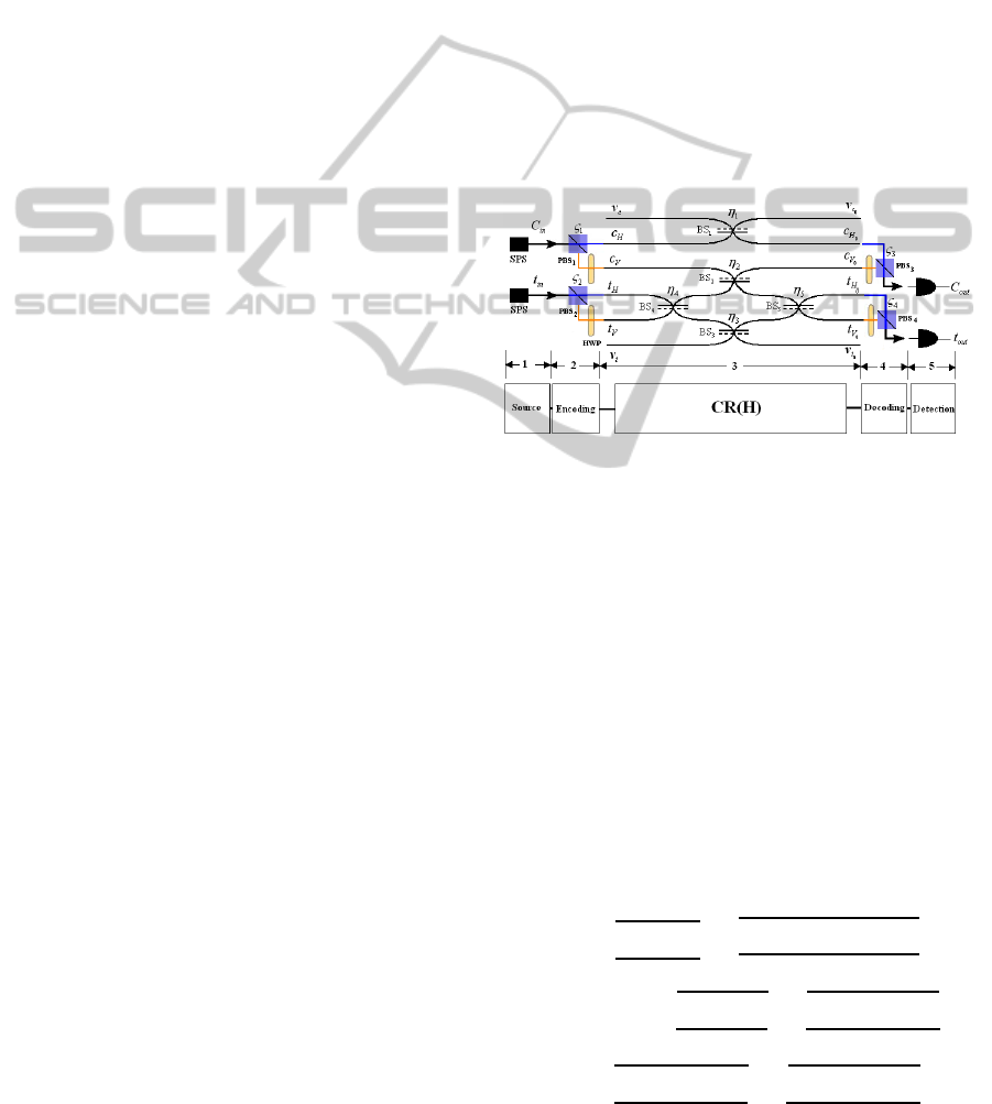
A generalization of the Ralph CNOT model is the
central componentillustrated by stage 3 of Figure 5. It
includes five Beam Splitters (BS), denoted BS
1
, BS
2
,
BS
3
BS
4
and BS
5
, characterized by five reflectivity co-
efficients η
1
, η
2
, η
3
, η
4
and η
5
, respectively. We de-
note the generalized CNOT Ralph model by CR(H),
where H = (η
1
, η
2
, η
3
, η
4
, η
5
) ∈ ]−1,1[
5
. The asso-
ciatedCNOT transfer matrix obtained from the circuit
is denoted by U
CR(H)
.
The encoding and decoding modules contains four
Polarizing Beam Splitter (PBS) and four Half Wave
Plate (HWP).
Figure 5: Generalization of the CNOT gate of TC.Ralph.
CR(H)operates on the dual rail coding to realize
the CNOT function.
Recall that in their work, TC.Ralph et al (Ralph
et al., 2002) used reflectivity coefficient η = η
1
=
η
2
= η
3
=
1
/3 and η
′
= η
4
= η
5
=
1
/2 and showed that
the CNOT gate operates with a success probability of
1
/9.
In the reality, BS imperfection of realization can’t
produce the values η =
1
/3, η
′
=
1
/2 but only values
that are closed to them. Since (
1
/3,
1
/2) are supposed
to be the ideal values, CR(H) is proposed.
Proposition.
A
p,ε
is realizable by CR(H), for H = (η
1
, η
2
, η
3
,
η
4
, η
5
) ∈ ]0,1[
5
, if the following equalities are satis-
fied:
p
1
=
√
η
1
η
2
η
4
η
5
+
p
η
1
η
3
(1−η
4
)(1−η
5
)
p
2
=
√
η
1
η
3
η
4
η
5
+
p
η
1
η
2
(1−η
4
)(1−η
5
)
p
3
= (1−2η
2
)
p
(1−η
4
)η
5
+
p
η
2
η
3
η
4
(1−η
5
)
p
4
= (1−2η
2
)
p
η
4
(1−η
5
) +
p
η
2
η
3
(1−η
4
)η
5
ε
1
=
p
η
1
η
2
(1−η
4
)η
5
−
p
η
1
η
3
η
4
(1−η
5
)
ε
4
=
p
η
1
η
2
η
4
(1−η
5
) −
p
η
1
η
3
(1−η
4
)η
5
SuccessProbabilityEvaluationofQuantumCircuitsbasedonProbabilisticCNOT-Gates
381

ε
9
= (1−2η
2
)
√
η
4
η
5
−
p
η
2
η
3
(1−η
4
)(1−η
5
)
ε
12
= (1−2η
2
)
p
(1−η
4
)(1−η
5
) −
√
η
2
η
3
η
4
η
5
p
1
=
√
η
1
η
2
η
4
η
5
+
p
η
1
η
3
(1−η
4
)(1−η
5
)
ε
j
1≤j≤12, j6={1,4,9,12}
= 0 (12)
Moreover, A
p,ε
is α-realizable ∀α ≥ 1 by CR(H),
where H = (η, η, η, η
′
, η
′
) ∈ ]0, 1[
5
, if η =
1
/3 and
η
′
=
1
/2.
Proof.
We consider η
BS
∈]0,1[ the reflectivity coefficient
of a BS. Let a
BS
in
, b
BS
in
be the two incoming photons
of the BS and a
BS
out
, b
BS
out
the outgoing photons. The
Heisenberg equation relating outputs-inputs are illus-
trated by Figure 6 (reflection upon dashed lines intro-
duces a π phase shift).
Figure 6: Heisenberg equation of the BS.
We consider the Heisenberg equations relating the
control (c
H
, c
V
) and target (t
H
, t
V
) inputs photons to
their corresponding outputs, depending on η
1
, η
2
, η
3
,
η
4
and η
5
(Figure 5). After excluding auxiliary inputs
ν
c
, ν
t
and outputs ν
c
0
, ν
t
0
, these equations are given
by the following:
c
H
0
=
√
η
1
c
H
+
p
(1−η
1
)v
c
c
V
0
= −
√
η
2
c
V
+
p
(1−η
2
)η
4
t
H
+
p
(1−η
2
)(1−η
4
)t
V
t
H
0
=
h
√
η
2
η
4
η
5
+
p
η
3
(1−η
4
)(1−η
5
)
i
t
H
+
h
p
η
2
(1−η
4
)η
5
−
p
η
3
η
4
(1−η
5
)
i
t
V
+
p
(1−η
2
)η
5
c
V
+
p
(1−η
3
)(1−η
5
)v
t
t
V
0
=
h
p
η
2
η
4
(1−η
5
) −
p
η
3
(1−η
4
)η
5
i
t
H
+
h
√
η
3
η
4
η
5
+
p
η
2
(1−η
4
)(1−η
5
)
i
t
V
+
p
(1−η
2
)(1−η
5
)c
V
−
p
(1−η
3
)η
5
v
t
(13)
For H = (η
1
, η
2
, η
3
, η
4
, η
5
) and s, t∈ N
∗
, these
equations permits to determine the transfer matrix
U
CR(H)
= (u
s,t
)
s,t≤4
as follows:
The input state |00i is represented by a presence
of a photon in |c
H
i and |t
H
i, the amplitude probability
of having the correct output |00i, meaning a simulta-
neous detection (coincidence basis) in |c
H
0
i and |t
H
0
i,
is given by the product of amplitude probabilities of
having a photon in |c
H
0
i and |t
H
0
i, when |c
H
i = |1i
and |t
H
i = |1i. Therefore, the resulting probability
amplitude u
1,1
is expressed as:
u
1,1
=
√
η
1
η
2
η
4
η
5
+
p
η
1
η
3
(1−η
4
)(1−η
5
)
The amplitude probability of having the erroneous
output |01i, |10i and |11i, meaning a simultaneous
detection on |c
H
0
i and |t
V
0
i, |c
V
0
i and |t
H
0
i , |c
V
0
i and
|t
V
0
i, are u
2,1
, u
3,1
and u
4,1
, respectively, expressed as:
u
2,1
=
p
η
1
η
2
(1−η
4
)η
5
−
p
η
1
η
3
η
4
(1−η
5
)
u
3,1
= 0, u
4,1
= 0
Following the same manner, the input state |01i
gives u
2,2
= p
2
, u
1,2
= ε
4
, u
3,2
= ε
5
, u
4,2
= ε
6
, the
input state |10i gives u
4,3
= p
3
, u
1,3
= ε
7
, u
2,3
= ε
8
,
u
3,3
= ε
9
and the input states |11i gives u
3,4
= p
4
,
u
1,4
= ε
10
, u
2,4
= ε
11
, u
4,4
= ε
12
, where (p
i
)
1≤i≤4
and
(ε
j
)
1≤j≤12
are expressed by equation 12.
We consider p = (p
1
, p
2
, p
3
, p
4
) and ε =
(ε
1
,0,0, ε
4
,0,0, ε
9
,0,0, ε
12
) a set of amplitude prob-
abilities depending on η
1
, η
2
, η
3
, η
4
and η
5
. U
CR(H)
defines a set of abstract probabilistic CNOT matrix
having the following form:
A
p,ε
=
p
1
ε
4
0 0
ε
1
p
2
0 0
0 0 ε
9
p
4
0 0 p
3
ε
12
(14)
Where A
p,ε
= U
CR(H)
.
We suppose that A
p,ε
is α-realizable ∀α ≥ 1 and
as requested by Ralph, η=η
1
=η
2
=η
3
, η
′
=η
4
=η
5
. En-
coding and decoding parts are supposed to operate
perfectly. According to these considerations, U
CR(H)
becomes:
U
CR(H)
=
η 0 0 0
0 η 0 0
0 0 −η+ η
′
(1−η) (1−η)
p
(1−η
′
)η
′
0 0 (1−η)
p
(1−η
′
)η
′
−η+ (1−η)(1−η
′
)
(15)
Moreover, by substituting these considerations
into equation 12, we deduce that p and ε becomes:
p
1
= p
2
= η
p
3
= p
4
= (1−η)
p
(1−η
′
)η
′
ε
9
= ε
12
−η+η
′
(1−η); ε
12
= −η+(1−η)
1−η
′
ε
j
1≤j≤11, j6=9
= 0 (16)
OPTICS2012-InternationalConferenceonOpticalCommunicationSystems
382
∀α ≥ 1, A
p,ε
of equation 16 is α-realizable if ε
9
=
0 and ε
12
= 0. Under these conditions, we deduce that
η =
1
/3 and η
′
=
1
/2.
4 ERRORS OF THE CNOT
RALPH MODEL
4.1 Internal Errors
We consider in the following errors affecting all BSs
composing stage 3 of figure 5.
BS reflectivity coefficient presents some uncer-
tainties with current BS technology. Work presented
in (Ralph et al., 2002) predicted an error of about
0.007 on BS reflectivity coefficient and it concluded
that errors below 0.01 are realistic. In the sequel, we
assume this error lower than 0.05.
We study in the following the influence of the
BSs errors on the α-realizability of A
p,ε
.
First Case:
For the ideal Ralph model, meaning η = η
1
= η
2
=
η
3
=
1
/3 and η
′
= η
4
= η
5
=
1
/2, we suppose that com-
mon error ξ ∈[−0.05,0.05] affects BS1, BS2 and BS3
and ξ
′
∈ [−0.05,0.05] affects BS4 and BS5, meaning
that η =
1
/3 + ξ and η
′
=
1
/2 + ξ
′
. Under these suppo-
sitions, p and ε of equation 16 changes as follows:
p
1
=
1
/3 + ξ
p
3
= (
2
/3 −ξ)
p
(
1
/2 −ξ
′
)(
1
/2 + ξ
′
)
ε
9
= −
3
2
ξ+
2
3
ξ
′
−ξξ
′
;ε
12
= −
3
2
ξ−
2
3
ξ
′
+ ξξ
′
(ε
j
)
1≤j≤11, j6=9
= 0 (17)
According to equations 17, a set of α-realizable
A
p,ε
transforms is defined for |p
1
| > α|ε
9
|, |p
1
| >
α|ε
12
|, |p
2
| > α|ε
9
| and |p
2
| > α|ε
12
|.
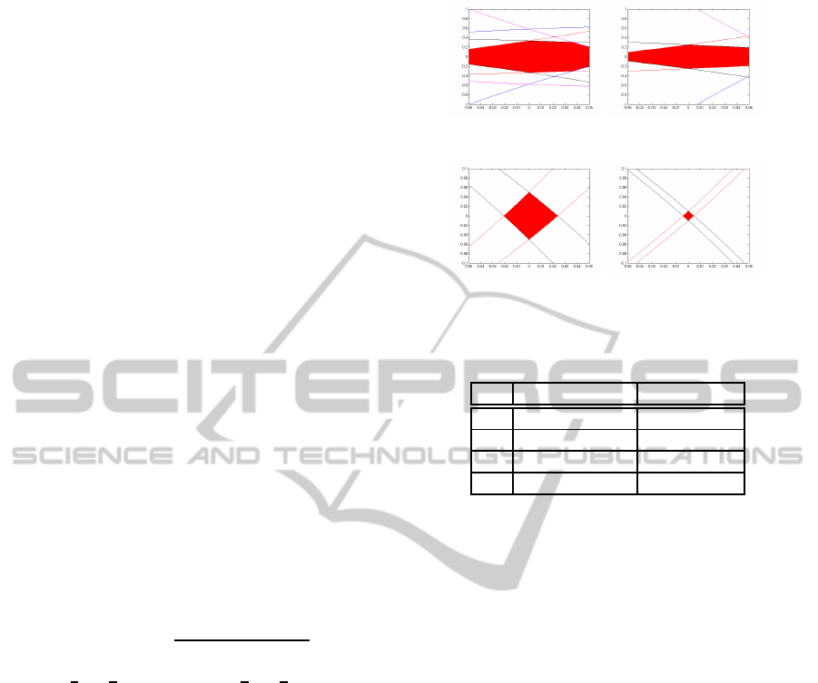
We vary ξ in [−0.05,0.05] and α in
{1.5, 2,10, 50}. The delimited area illustrated
by Figure 7(a), 7(b), 7(c) and 7(d), gives a represen-
tation of the parameters p and ε, for which A
p,ε
is
α-realizable by CR
(H)
.
According to Figure 7, α-realizability of A
p,ε
is
defined by the ranges of ξ and ξ
′
inside the intersec-
tion. Table 1 shows the range of the smallest rect-
angle containing the surfaces of interest that allows
α-realizability.
Second Case:
Even in the case where same technology is used
to construct BS1, BS2, BS3, BS4 and BS5, different
(a) α=1.5. (b) α=2.
(c) α=10. (d) α=50.
Figure 7: α-realizability of A
p,ε
depending on BSs errors.
Table 1: ξ and ξ
′
ranges defining α-realizable A
p,ε
.
α ξ ξ
′
1.5 [−0.05,0.05] [−0.05,0.05]
2 [−0.05,0.05] [−0.05,0.05]
10 [−0.021,0.023] [−0.05,0.05]
50 [−0.005,0.005] [−0.01,0.01]
errors occurs independently on η
1
, η
2
, η
3
, η
4
and η
5
,
respectively.
We consider (ξ
1
,ξ
2
,ξ
3
,ξ
4
,ξ
5
) ∈ ]−0.05,0.05[
5
the errors affecting optimal values (
1
/3,
1
/2) as:
(η
i
=
1
/3 +ξ
i
)
1≤i≤3
;
η
j
=
1
/2 +ξ
j
1≤j≤2
(18)
By substituting equations 18 into equations 12, we
obtain a set of A
p,ε
that are α-realizable and has the
form of equation 14.
Similarly to the process applied to common errors
(ξ and ξ
′
), one can use numerical simulation to build
Table 2 that illustrates the ranges of ξ
1
, ξ
2
, ξ
3
, ξ
4
and
ξ
5
, yielding to the smallest area permitting to get a set
of α-realizable A
p,ε
.
It’s worth to notice from this study that if we want
that A
p,ε
be α-realizable for high α values, then errors
should be minimal.
4.2 Input-output Errors
Encoding module in Figure 5 is composed of two
PBSs and two HWPs, this permits to move from po-
larization to dual rail encoding where the presence of
the single photon on the upper or the lower arms de-
fines the |0i and |1i states, respectively. The transfer
matrix of the encoding part is denoted by U
end
.
Decoding module of Figure 5 realizes the inverted
process and has a transfer matrix denoted by U
dec
.
SuccessProbabilityEvaluationofQuantumCircuitsbasedonProbabilisticCNOT-Gates
383
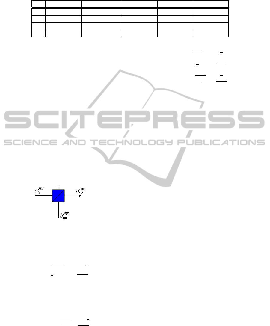
Table 2: ξ
1
, ξ
2
, ξ
3
, ξ
4
and ξ
5
ranges defining α-realizable A
p,ε
transform.
α ξ
1
ξ
2
ξ
3
ξ
4
ξ
5
1.5 [−0.05,0.05] [−0.05,0.05] [−0.05,0.05] [−0.05,0.05] [−0.05,0.05]
2 [−0.05,0.05] [−0.05,0.05] [−0.05,0.05] [−0.05,0.05] [−0.05,0.05]
10 [−0.05,0.05] [−0.03,0.03] [−0.05,0.05] [−0.05, 0.05] [−0.05,0.05]
50 [−0.05,0.05] [−0.001,0.001] [−0.02,0.02] [−0.01,0.01] [−0.01,0.01]
The encoding and decoding parts associated with
CR(H) previously studied, constitutes a polarization
encoding CNOT gate that is used to construct proba-
bilistic CNOT-based circuits.
The total transform of the CNOT gate, including
encoding and decoding part, is denoted by U
enc,dec
CR(H)
and obtained as follows:
U
enc,dec
CR(H)
= U
dec
.U
CR(H)
.U
enc
(19)
CR
(H)
of Figure 5 uses encoding-decoding mod-
ules, these latter may introduce errors due to imper-
fect PBS (Tyan et al., 1996). In our study, we neglect
errors that may be introduced by HWP since it does
not affect the logic function of the gate but rather it’s
second one, which is entangled photons state genera-
tion.
We denote a
PBS
in
the incoming photon of the PBS
(Figure 8) and a
PBS
out
, b
PBS
out
the outgoing photons.
Figure 8: Polarizing Beam Splitter with error.
The error introduced by the PBS is modeled by
ς ∈ [0,1], the PBS acts on the incident Horizontal (H)
and vertical (V) photons as follows:
a
PBS
in,H
→
p
1−ςa
PBS
out,H
+
√
ςb
PBS
out,H
(20)
a
PBS
in,V
→
√
ςa
PBS
out,V
+
p
1−ςb
PBS
out,V
In the two dimensional real vector space spanned
by the basis {|0i,|1i} with components |0i =
1 0
t
and |1i =
0 1
t
, the function of the
PBS is given as:
f
PBS
:
|0i →
√
1−ς|0i+
√
ς|1i
|1i →
√
ς|0i+
√
1−ς|1i
(21)
The matrix transform describing the PBS function
with error ς ∈ [0, 1], for h0| and h1| representing the
bras vectors and having matrix expression (10) and
(01), respectively, is denoted by U
ς
PBS
and given as:
U
ς
PBS
=
p
1−ς|0i+
√
ς|1i
h0|
+
√
ς|0i+
p
1−ς|1i
h1|
=
√
1−ς
√
ς
√
ς
√
1−ς
(22)
We consider ς
1
, ς
2
, ς
3
and ς
4
, the error introduced
by PBS1, PBS2, PBS3 and PBS4, respectively. By
considering parallel combining of PBS1 and PBS2,
parallel combining of PBS3 and PBS4, U
enc
and U
dec
are obtained as:
U
enc
= U
ς
1
PBS1
⊗U
ς
2
PBS2
; U
dec
= U
ς
3
PBS3
⊗U
ς
4
PBS4
Using the expression of U
enc
and U
dec
, one can
deduce U
enc,dec
CR(H)
by simple computation.
Let us show know that the transfer matrix pro-
vided experimentally by J.L.O.Brein (Brien et al.,
2003) can be computed with U
enc,dec
CR(H)
using specific
values for the errors. Since the values are hardly com-
plicated to obtain, we only show that we can approx-
imate closely the matrix P
Imp
CNOT
by selecting a series
of values. For example, if we take η
1
=
1
/3 −0.005,
η
2
=
1
/3 + 0.015, η
3
=
1
/3 −0.02, η
4
=
1
/2 + 0.04,
η
5
=
1
/2 + 0.05, ς
1
= 10
−3.2
, ς
2
= 10
−2
, ς
3
= 10
−2
and ς
4
= 10
−2
, then a direct computation of U
enc,dec
CR(H)
is obtained and the associated probability matrix, de-
noted by P
enc,dec
CR(H)
is given as:
P
enc,dec
CR(H)
=
0.1091 0.0051 0.0003 0.0011
0.0061 0.1080 0.0011 0.0001
0.0012 0.0002 0.0060 0.0970
0.002 0.0011 0.0969 0.0005
Knowing the expression of P
Imp
CNOT
(Brien et al.,
2003) which is equal to:
P
Imp
CNOT
=
0.1056 0.0034 0.0006 0.0012
0.0026 0.1044 0.0012 0.0001
0.0027 0.0002 0.0256 0.08
0.0001 0.0024 0.0833 0.0289
One can deduce that the approximation is in the
order of 10
−2
. A similar computation for other errors
values could show that P
enc,dec
CR(H)
is close to P
Imp
CNOT
in
lower order.
OPTICS2012-InternationalConferenceonOpticalCommunicationSystems
384
It’s worth to mention that in their implementation,
J.L.O.Brein et al (Brien et al., 2003)used as a Sin-
gle Photon Source (SPS) a pairs of energy degen-
erate photons generated through beam-like sponta-
neous parametric down-conversion and collected into
single-mode optical fibers (stage 1 of Figure 5), at the
output level (stage 5 of Figure 5), C
out
and t
out
are an-
alyzed by a system ending with a single photon count-
ing module (SPCM).
Let us finally notice that SPS and SPCM, accord-
ing to (Brida et al., 2006; Eiseman et al., 2011), do
introduce some extra errors that are not under investi-
gation in this work.
5 TOWARDS QUANTUM
ALGORITHM SIMULATION
5.1 Computation Scheme
A quantum algorithm whose circuit is acting on a
set of n qubits is a collection of binary functions
f
j
: {0,1}
n
→ {0,1}
n
, j = [1..x] where x ∈ N
∗
+
. The
quantum circuit realizing the algorithm which we de-
note by Qc
alg
, is composed by serial and parallel com-
bining of circuits realizing f
j
, denoted by Qc
f
j
. We
assume that Qc
f
j
is based on C
k
NOT gates.
Using the techniques developed in section 2.2, an
equivalent single qubit and CNOT gate based circuit
denoted by QC
CNOT
may be obtained. QC
alg
and
QC
CNOT
compute the same transfer matrix U
alg
. We
describe briefly in the following, several techniques
used to determine U
alg
.
An abstract probabilistic CNOT gate, acting on
two qubits is represented by Figure 9a. Study of
probabilistic CNOT-based quantum circuits requires
description of the abstract probabilistic CNOT trans-
form in multiple qubits system (Figure 9b) composed
of m + 2 qubits, where m ∈ N. To this end, A
p,ε
will
have the equivalent block matrix representation:
A
p,ε
≡
A
(1,1)
A
(1,2)
A
(2,1)
A
(2,2)
(23)
A
(1,1)
=
p
1
ε
4
ε
1
p
2
, A
(1,2)
=
ε
7
ε
10
ε
8
ε
11
,
A
(2,1)
=
ε
2
ε
5
ε
3
ε
6
and A
(2,2)
=
ε
9
p
4
p
3
ε
12
.
For m qubits between the control and the target ,
the effect on the final transform, depending on m, is
denoted by A
p,ε
(m) and obtained as:
A
p,ε
(m) =
I
⊗m
2
⊗A
(1,1)
I
⊗m
2
⊗A
(1,2)
I
⊗m
2
⊗A
(2,1)
I
⊗m
2
⊗A
(2,2)
(24)
Figure 9: CNOT gate used with m+ 2 qubits.
Using equation 24 and methods presented in
(Chakrabarti and Kolay, 2008; Shende et al., 2003),
we can use serial and parallel combining to determine
U
alg
by using identical CR(H) in all the circuit.
U
alg
is a function of nine errors, they are ξ
1
, ξ
2
,
ξ
3
, ξ
4
, ξ
5
affecting BSs and ς
1
, ς
2
, ς
3
, ς
4
affecting
PBSs. A control of the errors may provide a better
approximation of the algorithm function. We consider
this in more details in the next paragraph.
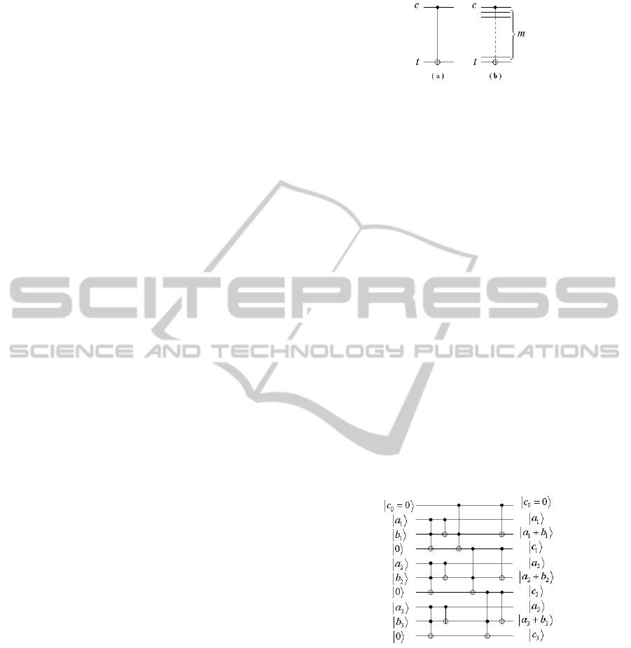
5.2 Case Study
Several proposal of Quantum adder circuits were pro-
posed in (Nakahara and Ohmi, 2008; Bannerjee and
Pathak, 2009; Kaye, 2004; Florio and Picca, 2004;
Vedral et al., 1996).The system used for our study
is the three qubits Minimized Quantum Ripple Carry
Adder (MQRCA) (Chakrabarti and Kolay, 2008). The
3-qubits MQRCA circuit is presented by Figure 10,
it computes the SUM of two numbers A and B,
represented by three qubits each as |a
3
,a
2
,a
1
i and
|b
3
,b
2
,b
1
i, respectively.
Figure 10: 3-qubits CNOT based MQRCA.
The total number of CNOT gates composing the
MQRCA is 9 ×8+ 3 = 75. The result of MQRCA is
given by |c
3
, a
3
+ b
3
, a
2
+ b
2
, a
1
+ b
1
i.
We present simulation results describing the errors
effect on the success probability when realizing the
SUM of |Ai = |4i and |Bi = |7i.
Deterministic CNOT gate realizes the addition
with certainty as illustrated by Figure 11(a).
When using CR(H), in one hand, we vary only
BSs errors for fixed (ς
1
,ς
2
,ς
3
,ς
4
) = (0,0, 0,0) as il-
lustrated by Table 3, in the other hand, we vary
PBSs errors for fixed values (ξ
1
,ξ
2
,ξ
3
,ξ
4
,ξ
5
) =
SuccessProbabilityEvaluationofQuantumCircuitsbasedonProbabilisticCNOT-Gates
385

Table 3: Varying BSs errors.
α η η
′
ξ
1
ξ
2
ξ
3
ξ
4
ξ
5
ς
1
ς
2
ς
3
ς
4
P
11
6.55
1
/3
1
/2
0.05 -0.05 0.04 0.01 -0.01 0 0 0 0 4.45×10
−48
20.94
1
/3
1
/2
0.03 -0.01 -0.02 0.015 0.01 0 0 0 0 4.51×10
−52
40.65
1
/3
1
/2
-0.01 0.001 -0.02 -0.001 0.007 0 0 0 0 4.76×10
−52
∞
1
/3
1
/2
0 0 0 0 0 0 0 0 0 2.96×10
−52
Table 4: Varying PBSs errors.
α η η
′
ξ
1
ξ
2
ξ
3
ξ
4
ξ
5
ς
1
ς
2
ς
3
ς
4
P
11
6.01
1
/3
1
/2
0.05 -0.05 0.04 0.01 -0.01 10
−4.1
10
−4
10
−4.5
10
−3.8
5.15×10
−48
5.8
1
/3
1
/2
0.05 -0.05 0.04 0.01 -0.01 10
−3
10
−3.2
10
−3.4
10
−3.5
8.41×10
−48
4.66
1
/3
1
/2
0.05 -0.05 0.04 0.01 -0.01 10
−2
10
−2.2
10
−2.4
10
−2.5
1.8×10
−44
(a) Ideal CNOT. (b) α = ∞.
(c) α = 6.55. (d) α = 20.94. (e) α = 40.65.
(f) α = 6.01. (g) α = 5.8. (h) α = 4.66.
Figure 11: Success probability of (4+ 7).
(0.05,−0.05, 0.04,0.01, −0.01) as illustrated by Ta-
ble 4.
U
CR(H)
associated to (ξ
1
, ξ
2
, ξ
3
, ξ
4
, ξ
5
)=(0.05,
−0.05, 0.04, 0.01, −0.01) and (ς
1
, ς
2
, ς
3
, ς
4
)=(0, 0,
0, 0) is given as follows:
U
CR(H)
= U
enc,dec
CR(H)
=
0.3539 −0.0173 0 0
−0.0314 0.3539 0 0
0 0 0.054 0.3804
0 0 0.3782 0.054
(25)
According to equation 25, α =
0.3539
/0.054 =6.55.
For different α values, the resulting success probabil-
ity of realizing correctly the SUM 4+7, denoted by
P
11
, is illustrated by Figure 11.
The correct output is obtained for probability P
11
around 10
−52
, which is significant comparing to the
other outputs
10
−54
, but non interesting for realiz-
ing arithmetic operations.
We notice that this probability is very low since
the success probability of the used model is around
1
/9, the success probability decreases exponentially
depending on the number of probabilistic CNOT
gates used (=75).
Figures 11(b), 11(c), 11(d) and 11(e) shows the re-
sult of the SUM for α = [∞,6.55,20.94,40,65]. This
figure shows that the higher the α value, the higher is
the GAP between P
11
and non significant results, but
the lower is P
11
.
Figure 11(f), 11(g) and 11(h) illustrate the impact
of the encoding and decoding parts. ς
1
, ς
2
, ς
3
and ς
4
contribute to decrease α value and push non signifi-
cant results to be closer to P
11
. An upper bound to
keep detection possible in our case is approximated
to a PBS error around ζ = 10
−3
.
6 CONCLUSIONS
In this work, we have defined an abstract probabilis-
tic CNOT model, we identified and modeled errors
occurring in the success probability in the case of
T.C.Ralph CNOT based implementation. We also
studied the effect of the errors occurring in the imple-
mentation of quantum algorithm when it uses identi-
calCNOT called generalized RalphCNOT model and
abbreviated CR(H). The work we have performed
here, for CR(H) based technology can be used with
other technologies. We omitted in this paper to dis-
cuss the other technologies because of the lack of
space and the redundancy of results. We believe that
the study of implementations based on linear compo-
nents will highlight a large range of α-realizable ab-
stract probabilistic CNOT. Our future work address
this issue.
OPTICS2012-InternationalConferenceonOpticalCommunicationSystems
386

REFERENCES
Bannerjee, A. and Pathak, A. (2009). An analysis of re-
versible multiplier circuits. arXiv:0907.3357, pages
1–10.
Barenco, A., Bennett, C. H., Cleve, R., DiVincenzo, D. P.,
Margolus, N., Shor, P., Sleator, T., Smolin, J. A., and
Weinfurter, H. (1995). Elementary gates for quantum
computation. Phys. Rev. A, vol.52:pp.3457–3467.
Brida, G., Genovese, M., and Gramegna, M. (2006).
Twin photon techniques for photo-detector calibra-
tion. Laser.Phys.Lett, vol.3, no.3:115–123.
Brien, J. L. O., Pryde, G. J., White, A. G., Ralph, T. C., and
Branning, D. (2003). Demonstration of an all-optical
quantum controlled-not gate. Nature, vol.426:pp.264–
267.
Chakrabarti, A. and Kolay, S. S. (2008). Designing quan-
tum adder circuits and evaluating their error perfor-
mance. In International conference on Electronic de-
sign ICED2008, pages 1–6.
Eiseman, M. D., Fan, J., Migdall, A., and Polyavok,
S. s. (2011). Single photon sources and detectors.
Rev.Sci.Instrum, vol.82:p.071101.
Florio, G. and Picca, D. (2004). Quantum implementation
of elementary arithmetic operations. arXiv: quant-
ph/0403048.
Kaye, P. (2004). Reversible addition circuit using one an-
cillary bit with application to quantum computing.
arXiv: quant-ph/0408173v2.
Nakahara, M. and Ohmi, T. (2008). ”Quantum computing
from linear algebra to physical realizations”. CRC
Press, Taylor & Fancis Group, 6000 Broken sound
parkway NW, suite 300, Boca Raton, FL 33487-2742.
Okamoto, R., Hofmann, H. F., Takeuchi, S., and Sasaki,
K. (2005). Demonstration of an optical quantum con-
trolled not gate without path interference. Phys. Rev.
Lett.95, 210506:4 pages.
Pittman, T. B., Fitch, M. J., Jacobs, B. C., and Franson, J. D.
(2003). Experimental controlled not logic gate for
single photons in the coincidence basis. Phys.Rev.A,
vol.68:p.032316.
Pittman, T. B., Jacobs, B. C., and Franson, J. D. (2001).
Probabilistic quantum logic operations using polariz-
ing beam splitters. Phys.Rev.A, vol.64:p.062311.
Ralph, T. C., Langford, N. K., Bell, T. B., and White, A. G.
(2002). Linear optical controlled not gate in the coin-
cidence basis. Phys. Rev. A.65, 062324:5 pages.
Shende, V. V., Prasad, A. K., Markov, I. L., and Hayes, J. P.
(2003). synthesis of reversible logic circuits. IEEE
transaction on computer-aided design of integrated
circuits and systems, VOL 22, NO 6.
Tyan, R. C., Sun, P. C., and Tyan, Y. F. R.-C. (1996). Polar-
izing beam splitters constructed of form-birefringent
multilayer gratings. Proc. SPIE 2689, 82.
Vedral, V., Barenco, A., and Ekert, A. (1996). Quantum
networks for elementary arithmetic operations. Phys.
Rev. A., vol.54:pp.147–153.
SuccessProbabilityEvaluationofQuantumCircuitsbasedonProbabilisticCNOT-Gates
387
