
Global Visual Features based on Random Process
Application to Visual Servoing
Laroussi Hammouda
1
, Khaled Kaaniche
1,2
, Hassen Mekki
1,2
and Mohamed Chtourou
1
1
Intelligent Control Design and Optimization of Complex Systems, University of Sfax, Sfax, Tunisia
2
National School of Engineering of Sousse, University of Sousse, Sousse, Tunisia
Keywords: Visual Servoing, Global Visual Features, Mobile Robot.
Abstract: This paper presents new global visual features: random distribution of limited set of pixels luminance. Our
approach aims to improve the real-time performance of visual servoing applications. In fact, using these
new features, we reduce the computation time of the visual servoing scheme. Our method is based on a
random process which ensures efficient and fast convergence of the robot. The use of our new features
removes the matching and tracking process. Experimental results are presented to validate our approach.
1 INTRODUCTION
Computer vision is progressively playing more
important role in service robotic applications. In
fact, the movement of a robot equipped with a
camera can be controlled from its visual perception
using visual servoing technique. The aim of the
visual servoing is to control a robotic system using
visual features acquired by a visual sensor
(Chaumette and Hutchinson, 2008). Indeed, the
control law is designed to move a robot so that the
current visual features , acquired from the current
pose , will reach the desired features
∗
acquired
from the desired pose
∗
, leading to a correct
realization of the task.
The control principle is thus to minimize the
error = −
∗
where is a vector containing the
current values of the chosen visual information, and
∗
its desired values. The basic step in image-based
visual servoing is to determine the adequate set of
visual features to be extracted from the image and
used in the control scheme in order to obtain an
optimal behavior of the robot.
In the literature several works were concerned
with simple objects and the features used as input of
the control scheme were generally geometric:
coordinates of points, edges or straight lines (Espiau
and al., 1992), (Chaumette and Hutchinson, 2007).
These geometric features have always to be
tracked and matched over frames. This process has
proved to be a difficult step in any visual servoing
scheme. Therefore, in the last decade, the
researchers are focused on the use of global visual
features. In fact, in (Collewet and al., 2008) the
visual features considered are the luminance of all
image pixels and the control law is based on the
minimization of the error which is the difference
between the current and the desired image.
Others works are interested in the application of
image moments in visual servoing, like in
(Chaumette and Hutchinson, 2003) where the
authors propose a new visual servoing scheme based
on a set of moment invariants. The use of these
moments ensures an exponential decoupled decrease
for the visual features and for the components of the
camera velocity. However this approach is restricted
to binary images. It gives good results except when
the object is contrasted with respect to its
environment.
In (Dame and Marchand, 2009), the authors
present a new criterion for visual servoing: the
mutual information between the current and the
desired image. The idea consists in maximizing the
information shared by the two images. This
approach has proved to be robust to occlusions and
to very important light variations. Nevertheless, the
computation time of this method is relatively high.
The work of (Marchand and Collewet, 2010)
proposes the image gradient as visual feature for
visual servoing tasks. This approach suffers from a
small cone of convergence. Indeed, using this visual
feature, the robotic system diverges in the case of
large initial displacement. Another visual seroving
approach which removes the necessity of features
tracking and matching step has been proposed in
105
Hammouda L., Kaaniche K., Mekki H. and Chtourou M..
Global Visual Features based on Random Process - Application to Visual Servoing.
DOI: 10.5220/0004040701050112
In Proceedings of the 9th International Conference on Informatics in Control, Automation and Robotics (ICINCO-2012), pages 105-112
ISBN: 978-989-8565-22-8
Copyright
c
2012 SCITEPRESS (Science and Technology Publications, Lda.)

(Abdul Hafez and al., 2008). This method models
the image features as a mixture of Gaussian in the
current and in the desired image. But ,using this
approach, an image processing step is always
required to extract the visual features.
The contribution of this paper consists in the
definition of new global visual features: random
distribution of limited set of pixels luminance. Our
features improve the computation time of visual
servoing scheme and avoid matching and tracking
step. We illustrate in this work an experimental
analysis of the robotic system behavior in the case of
visual servoing task based on our new approach.
This paper is organized as follows: Section 2
illustrates our new visual features and the
corresponding interaction matrix. Section 3 recalls
the optimization method used in the building of the
control law. Finally, experimental results are
presented in section 4.
2 RANDOM DISTRIBUTION OF
LIMITED SET OF PIXELS
LUMINANCE AS VISUAL
FEATURES
The use of the whole image luminance as global
visual features for visual servoing tasks, as in
(Collewet and Marchand, 2011), requires too high
computation time. Indeed, the big size of the
interaction matrix related to the luminance of all
image pixels leads to a very slow convergence of the
robotic system.
Therefore, we propose in this paper a new visual
feature which is more efficient in terms of
computation time and doesn’t require any matching
nor tracking step.
In fact, instead of using the luminance of all
image points, we work just with the luminance of a
random distribution of a limited set of image points
( pixels). Thus, the visual features, at a position
of the robot, are:
()=
() (1)
with
() is the luminance of random set of image
pixels taken at frame .
(
)
=(
,
,
,….,
) (2)
where
is the luminance of the pixel taken
randomly at the frame .
For each new frame, we get a new random set of
image pixels. Thus, the desired and the current
visual features will continuously change along the
visual servoing scheme. In that case, the error e will
be:
=
(
)
−
∗
(
∗
)
(3)
where
(
)
represent the current visual features and
∗
(
∗
)
the desired ones at the frame .
Consequently, in our method, the error used in
the building of the control law is variable, it changes
at each frame. This change is like a kind of
mutation. Convergence to global minimum is then
guaranteed.
The choice of is based on the image histogram.
We take equal to the maximum value of the
current image histogram. We can then avoid the fact
that the pixels randomly chosen will have the
same luminance. Hence, we guarantee the good
luminance representation of the image. We note
the probability that the pixels will have the same
luminance. It is given by:
=
=
!
!
(
)
!
(4)
where is the number of pixels deduced from the
image histogram and chosen as visual features and
is the number of all image pixels. This probability is
null (see Table 1).
Since the number depends on the histogram of
the current image, it slightly changes during the
visual servoing scheme. Let us point that is always
very small compared to the total number of image
pixels (in our case 320×240). We note that the
more the image is textured, the smaller is.
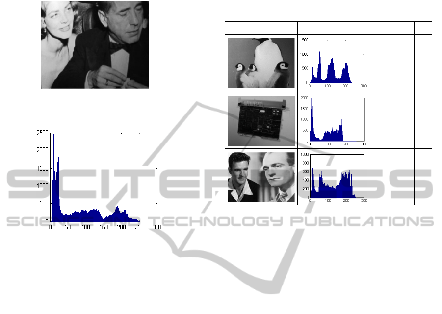
Figure 1 shows an example of image, the
luminance of all its pixels form the ancient global
visual features.
The histogram of this image is illustrated on
Figure 2. In our approach, instead of using all image
pixels, we take randomly pixels as global visual
features, with is the maximum value of this
histogram (in this example = 2452 which is 3.1%
of all image pixels).
After ensuring that the pixels are good
respresentatives of the image luminance, we can
confirm that these pixels randomly chosen will be
well distributed in the image and not concentred in
one particular zone. For that, we compute the
probability that the pixels will be all in one zone .
This probabilty is given by:
=
=
!
!
(
)
!
!
!
(
)
!
(5)
ICINCO2012-9thInternationalConferenceonInformaticsinControl,AutomationandRobotics
106
with is the number of pixels in a compact zone of
the image.
Figure 1: Ancient visual features: The whole image
luminance.
Figure 2: Image histogram (essential for the choice of ).
In our work, we take as the half of all image
pixels (Beyond this value of we assume that good
image representation is ensured).
The probability
is equal to zero (see Table 1).
This proves that the pixels chosen as visual
features will always ensure good spatial
respresentation of the scene.
We present in Table 1 the histograms and the
probabilities (
and
) related to different images.
The visual servoing is based on the relationship
between the robot motion and the consequent change
on the visual features. This relationship is expressed
by the well known equation (Chaumette and
Hutchinson, 2006):
=
(6)
where
is the interaction matrix that links the time
variation of to the robot instantaneous velocity
(Chaumette and Hutchinson, 2008).
So, after identification of the visual features, the
control law requires the determination of this matrix
which is at the center of the development of any
visual servoing scheme. In our case, we look for the
interaction matrix related to the luminance of a pixel
x in the image.
The computation of this matrix is based on the
optical flow constraint equation (OFCE) which is a
hypothesis that assumes the temporal constancy of
the luminance for a physical point between two
successive images (Marchand, 2007).
Table 1: Examples of images with the corresponding
histograms and probabilities.
Image Histogram
1089
0
0
1979 0 0
940 0 0
If a point x of the image realizes a displacement
x in the time interval , according to the previous
hypothesis we have:
(x+x,+)=(x,) (7)
After development of this equation we get:
∇
x +
=0 (8)
where
=
()
and ∇ is the spatial gradient of x.
We know that: x =
(9)
where
is the interaction matrix that relates the
temporal variation of x to the control law.
Using (8) and (9) we obtain:
=−
(10)
So the interaction matrix that relates the temporal
variation of the luminosity (x) to the control law
is:
()
=−∇
(11)
In this case, we can write the interaction matrix
()
in terms of the interaction matrices
and
related to the coordinates of x=(,) and we
obtain:
()
=−(∇
+∇
) (12)
with ∇
are the components along x and y of
∇(x).
In the case of a mobile robotic system, we take
into account just the components of
that
correspond to three degrees of freedom: Translation
GlobalVisualFeaturesbasedonRandomProcess-ApplicationtoVisualServoing
107

along axis, translation along axis and rotation
around axis. Therefore, we have:
=(−
−
(
1+
)
) (13)
= (0
−) (14)
where is the depth of the point x relative to the
camera frame.
We get the interaction matrix related to our new
features (
) by combining the interaction matrices
related to the pixels randomly chosen.
Thus, the size of the interaction matrix related to
our visual features (
) is very small compared to
the size of the interaction matrix related to the whole
image luminance.
3 THE CONTROL LAW
GENERATION
In our work we use a global photometric visual
features .In this case most of classical control laws
fail. Therefore, we have interest in turning the visual
servoing scheme into an optimization problem to get
the convergence of the mobile robot to its desired
pose (Abdul Hafez and Jawahar, 2006), (Abdul
Hafez and Jawahar 2007). In fact, the aim of the
control law will be the minimization of a cost
function which is the following:
(
)
=
(
)
−
(
∗
)
(
(
)
−
(
∗
)
) (15)
where () are the current visual features (
(
)
)
and (
∗
)are the desired ones (
∗
(
∗
)
).
The cost function minimization is, essentially,
based on the following step:
=
⨁(
) (16)
where “⨁” denotes the operator that combines two
consecutive frame transformations,
is the current
pose of the mobile robot (at frame ),
is the next
pose of the mobile robot and (
) is the direction of
descent.
This direction of descent must ensure that
d
(
)
∇
(
)
<0. In this way, the movement of the
robot leads to the decrease of the cost function.
Optimization methods depend on the direction of
descent used in the building of the control law. The
control law usually used in visual servoing context is
given by:
=−
(
)
−
(
∗
)
(17)
where is a positive scalar and
is the pseudo
inverse of the interaction matrix.
This classical control law gives good results in
the case of visual servoing task based on geometric
visual features (Chaumette and Hutchinson, 2006).
Since we work with photometric visual features
this classical control law fails and doesn’t ensure the
convergence of the robot (Collewet and al., 2008).
Thus, in our work we use the control law based on
the Levenberg-Marquardt approach. The control law
generated to the robot, using our new features, is
then given by:
=−
+
(18)
where
is the error corresponding to these new
features:
=
(
)
−
∗
(
∗
)
(19)
and with
=
(20)
4 EXPERIMENTAL RESULTS
4.1 Experimental Environment
We present the results of a set of experiments
conducted with our visual features. All the
experiments reported here have been obtained using
a camera mounted on a mobile robot. In each case,
the mobile robot is first moved to its desired pose
∗
and the corresponding image
∗
is acquired. From
this desired image, we extract the desired visual
features
∗
. The robot is then moved to a random
pose and the initial visual features s are extracted.
The velocities computed, at each frame, using the
control law, are sent to the robot until its
convergence. The interaction matrix is calculated at
each frame of the visual servoing scheme. In a first
step we conduct our experiments on a virtual
platform of VRML, therefore we can recuperate, at
each frame, the pose of the mobile robot in terms of
position along two translational axes and around one
rotational axe. In a second step we validate our
results on a real mobile robot (Koala robot).
4.2 Interpretation
During the experiments conducted on the VRML
environment we take as initial positioning error:
∆r
=
(
18cm,12cm, 9°
)
. We illustrate the
results obtained using our new visual features on
ICINCO2012-9thInternationalConferenceonInformaticsinControl,AutomationandRobotics
108
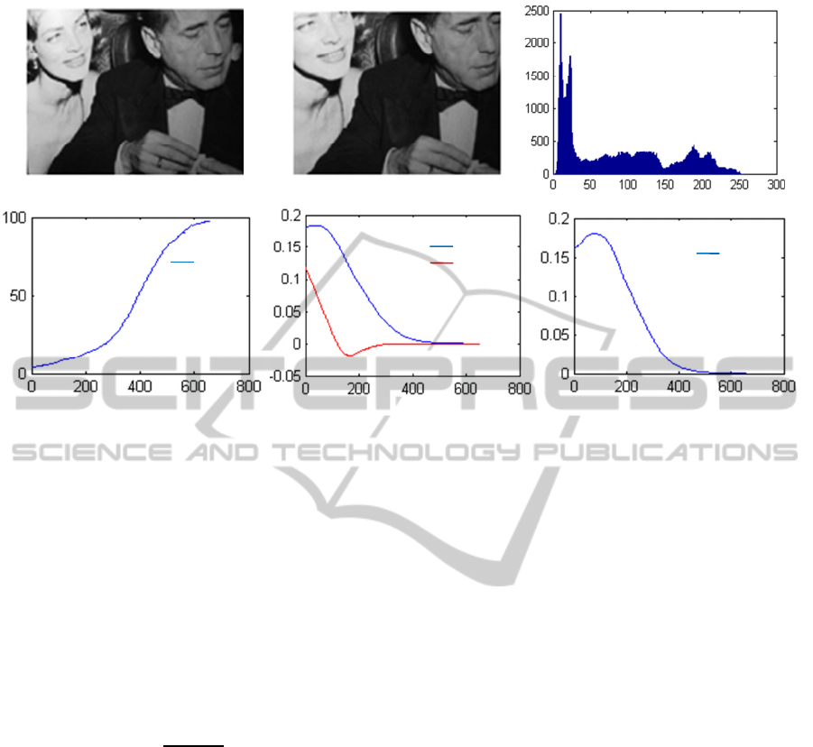
Figure 3: First experiment with our new global visual features (x axis in frame number for (d), (e) and (f)): (a) Initial image,
(b) Desired image, (c) Initial image histogram, (d) Stopping criterion evolution: () in percentage (%), (f) Translational
positioning errors: ∆ and ∆ in meter (), (f) Rotational positioning error: ∆ in radian ().
Figures 3 and 4 (first and second experiment).
Figures 3a and 4a present the initial scenes.
Figures 3b and 4b depict the desired scenes. The
histograms of the initial images are shown on
Figures 3c and 4c.
We choose as stopping criterion of our program
the following measure:
(
)
which is the proportion
of the number of pixels, in the error image (−
∗
),
whose luminance is below a certain threshold
compared to the total number of image pixels.
(
)
=
()
×100 (21)
where
() is the number of pixels in the error
image whose luminance is below a predefined
threshold at pose of the robot and
is the
total number of pixels (320×240).
In our experiments we choose the luminance
value 3 as a threshold. We suppose that the
convergence is achieved and the robotic system
reaches its desired pose when
(
)
get at 98%.
Figures 3d and 4d depict the behavior of this
stopping criterion. The translational positioning
errors
(
∆,∆Tz
)
between the current and the
desired pose during the positioning task are shown
on Figures 3e and 4e. The rotational positioning
errors
(
∆
)
are illustrated on Figures 3f and 4f.
We note that the robotic system converges with
good
behaviour using our global visual features
(
(
)
=
(
)
) and it spend very less time compared
to the method of (Collewet and al., 2008).
Indeed, our method reduces the size of the visual
features vector . Thus, the size of the interaction
matrix related to our visual features (
) is very
small compared to the size of the interaction matrix
related to the whole image luminance. Therefore,
our approach is more suitable to real-time
applications. As an example, the experiment of
Figure 3 has demonstrated that, using our approach,
the computation time for each 320×240 frame
does not exceed 40 ms while it is 270 ms when we
work with the whole image luminance as visual
features.
After using the virtual platform of VRML, we
validated our new approach using the Koala mobile
robot which is a differential wheeled robot. The
results of the experiments conducted on the Koala
are illustrated on Figure 5. We remark that this
mobile robot correctly converges to its desired pose
using our new global visual features. The initial and
the desired scene are reported respectively on
Figures 5a and 5b. The evolutions of the velocities
of the two robot wheels are illustrated on Figure 5c
where
is the right wheel and
is the left one.
The stopping criterion evolution is shown on Figure
5d. So, we can confirm that our new visual features
give good results in the case of real conditions of
visual servoing task.
(a) (b) (c)
(d) (e) (f)
∆
∆
∆
()
GlobalVisualFeaturesbasedonRandomProcess-ApplicationtoVisualServoing
109
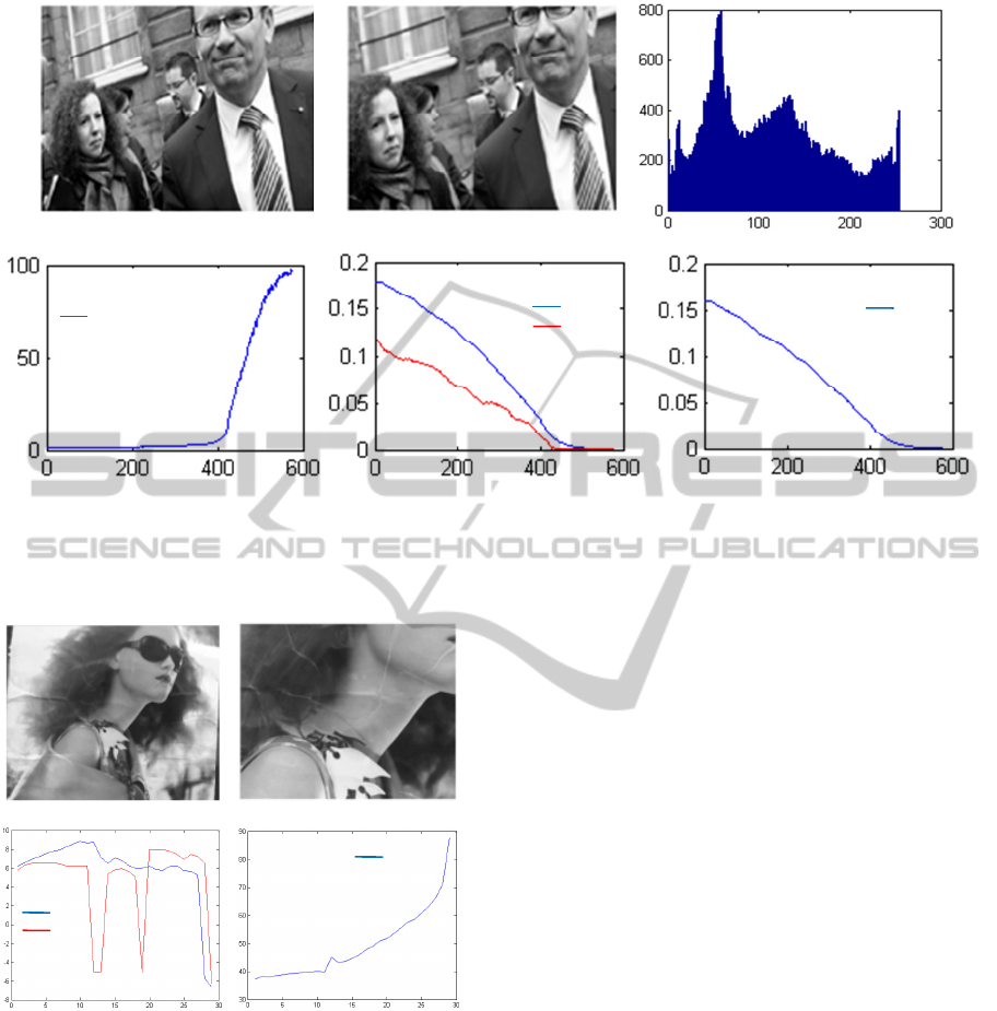
Figure 4: Second experiment with our new global visual features (x axis in frame number for (d), (e) and (f)): (a) Initial
image, (b) Desired image, (c) Initial image histogram, (d) Stopping criterion evolution: () in percentage (%),
(f) Translational positioning errors: ∆ and ∆ in meter (), (f) Rotational positioning error: ∆ in radian ().
Figure 5: Our global visual features (axis in frame
number). (a) Initial scene, (b) Desired scene, (c) The
velocities of the two robot wheels (/), (d) Stopping
criterion evolution: ()(%).
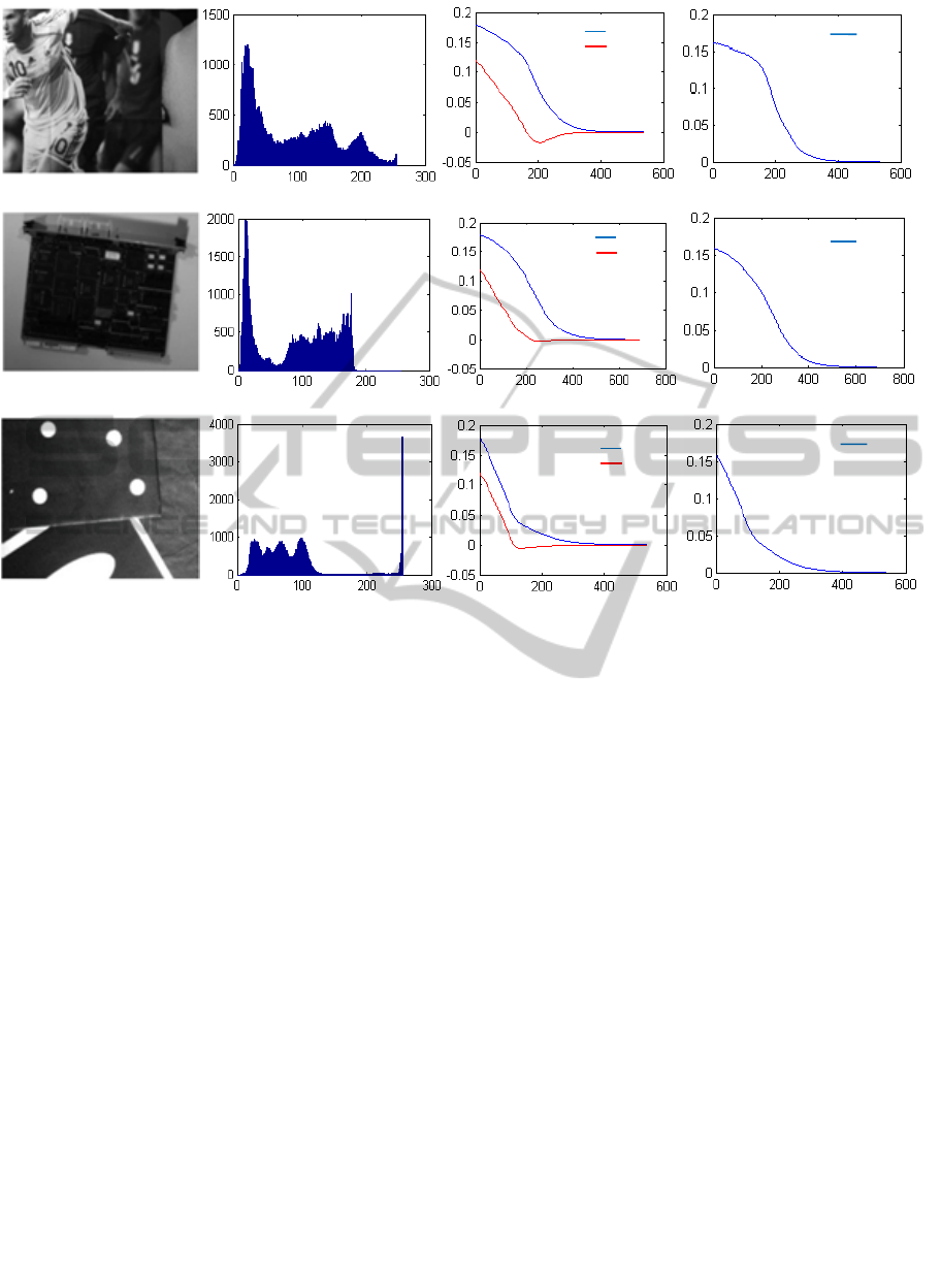
4.3 Robustness with Respect to Image
Content
Our approach does not depend on the image content.
In fact, the experiments demonstrate that the control
law converges even in the case of low textured
scenes.
Figure 6 shows that using different types of
scenes the control law converges in all the cases (we
keep the same initial positioning errors). The images
presented here are those used in (Collewet and al.,
2010).
The first column in Figure 6 shows the different
scenes. The second represents the corresponding
histograms. The third and the fourth column
illustrate, respectively, the translational and the
rotational positioning errors during the visual
servoing scheme.
5 CONCLUSIONS
In this paper we focused on the importance of global
visual features in visual servoing applications.
We found that when the used global feature is the
whole image luminance the mobile robot takes so
much time to reach its desired pose, therefore we
proposed a new approach to achieve fast and real-
time visual servoing tasks. This approach is based on
new global feature which is the luminance of a
random distribution of image points. To demonstrate
the efficiency of this new method our works were,
firstly, realized on a virtual platform of VRML then
on a real mobile robot. To get the convergence of the
robot we have turned the visual servoing problem
into an optimization problem. Thus, we have used
(a) (b) (c)
(d) (e) (f)
()
(d) (c)
(a)
(b)
∆
∆
∆
()
ICINCO2012-9thInternationalConferenceonInformaticsinControl,AutomationandRobotics
110
(a) (b) (c) (d)
(e) (f) (g) (h)
(i) (j) (k) (l)
Figure 6: Results of our approach in different cases of scenes. First column: scenes considered, second column:
corresponding histograms, third column: translational positioning errors in meter (x axis in frame number), fourth column:
rotational positioning errors in radian (x axis in frame number).
the control law based on the minimization of a cost
function since that ensures the convergence in the
case of global visual features.
The new feature has proved to be able to ensure
good and fast convergence of the mobile robot even
in the case of low textured scenes. As it is global, it
does not require any matching nor tracking step and
there is no image processing step.
Future works can be intended to verify the
robustness of our approach with respect to partial
occlusions and large illumination changes.
REFERENCES
Abdul Hafez A., Achar S., and Jawahar, C., 2008. Visual
servoing based on Gaussian mixture models. In IEEE
Int. Conf. on Robotics and Automation, Pasadena,
California, pp 3225–3230.
Abdul Hafez, A., and Jawahar, C., 2006. Improvement to
the minimization of hybrid error functions for pose
alignement, in IEEE Int. conf. on Automation
Robotics, Control and Vision, Singapore.
Abdul Hafez, A.H., and Jawahar, C., 2007. Visual
Servoing by Optimization of a 2D/3D Hybrid
Objective Function. In IEEE International Conference
on Robotics and Automation, pp 1691 – 1696, Roma.
Chaumette, F., and Hutchinson, S., 2003. Application of
moment invariants to visual servoing. In IEEE Int.
Conf. on Robotics and Automation, pp 4276-4281,
Taiwan.
Chaumette, F., and Hutchinson, S., 2006. Visual servo
control, Part I: Basic approaches. In IEEE Robotics
and Automation Magazine, 13(4):82–90.
Chaumette, F., and Hutchinson, S., 2007. Visual servo
control, part II: Advanced approaches”. IEEE Robotics
and Automation Magazine, vol. 14, no. 1.
Chaumette, F., and Hutchinson, S., 2008. Visual servoing
and visual tracking”. In B. Siciliano and O. Khatib,
editors, Handbook of Robotics, chapter 24, pp. 563–
583. Springer.
Collewet, C., Marchand, E., and Chaumette, F.,
2008.Visual servoing set free from image processing.
In IEEE Int. Conf. on Robotics and Automation, CA,
pp. 81–86, Pasadena.
Collewet, C., Marchand, E., and Chaumette, F., 2010.
Luminance: a new visual feature for visual servoing.
In Visual Servoing via Advanced Numerical Methods
LNCIS 401, Springer-Verlag (Ed), 71—90.
Collewet, C., and Marchand, E., 2011. Photometric visual
servoing. In IEEE Trans. on Robotic, Vol. 27, No.4.
pp. 828-834.
∆
∆
∆
∆
∆
∆
∆
∆
∆
GlobalVisualFeaturesbasedonRandomProcess-ApplicationtoVisualServoing
111

Dame, A., Marchand, E., 2009. Entropy-based visual
servoing. In IEEE ICRA’09, pp. 707–713, Kobe,
Japan.
Espiau, B., Chaumette, F., and Rives, P., 1992. A new
approach to visual servoing in robotics. IEEE Trans.
on Robotics and Automation, 8(3):313-326.
Marchand, E., 2007. Control camera and light source
positions using image gradient information. In IEEE
Int. Conf. on Robotics and Automation, ICRA’07,
pages 417–422, Roma, Italia.
Marchand, E., and Collewet, C., 2010. Using image
gradient as a visual feature for visual servoing. In
IEEE/RSJ Int. Conf. on Intelligent Robots and
Systems, pp 5687-5692, Taiwan.
ICINCO2012-9thInternationalConferenceonInformaticsinControl,AutomationandRobotics
112
