
Support Vector Machines for Identification of HCCI Combustion
Dynamics
Vijay Manikandan Janakiraman
1
, Jeff Sterniak
2
and Dennis Assanis
3
1
Department of Mechanical Engineering, University of Michigan, Ann Arbor, MI, U.S.A.
2
Robert Bosch LLC, Farmington Hills, MI, USA
3
Stony Brook University, Stony Brook, NY, U.S.A.
Keywords:
Support Vector, Identification, Combustion, Homogeneous Charge Compression Ignition, HCCI, Neural
Networks, Nonlinear Regression, Engine Model, Control Model.
Abstract:
Homogeneous charge compression ignition (HCCI) is a promising technology for Internal Combustion En-
gines to improve efficiency and reduce nitrogen oxides emissions. Control of HCCI combustion is often
model-based, and it is vital to have a good model of the engine to make control decisions. The HCCI engine is
characterized by complex chemical kinetics whose physical modeling is difficult and laborious. Identification
is an effective alternative to quickly develop control oriented models for such systems. This paper formulates
a Support Vector Regression (SVR) methodology for developing identification models capturing HCCI com-
bustion behavior. Measurable quantities from the engine such as net mean effective pressure (NMEP) and
crank angle at 50% mass fraction burned (CA50) can be used to characterize and control the HCCI engine and
are considered for identification in this study. The selected input variables include injected fuel mass (FM)
and valve events {intake valve opening (IVO), exhaust valve closing (EVC)}. Transient data from a gasoline
HCCI engine recorded at stable HCCI conditions is used for training, validating and testing the SVR models.
Comparisons with the experimental results show that SVR with Gaussian kernels can be a powerful approach
for identification of a complex combustion system like the HCCI engine.
1 INTRODUCTION
In recent years, the requirements on automotive per-
formance, emissions and safety have become increas-
ingly stringent. In spite of advanced concepts enter-
ing the industry, achieving fuel economy, emission
and cost targets simultaneously still remains an ar-
duous task. HCCI engines gained the spotlight from
traditional spark ignited and compression ignited en-
gines owing to its ability to reduce emissions and fuel
consumption significantly (Thring, 1989; Christensen
and Johansson, 1997; Aoyama and Sato, 1996). In
spite of its known advantages, HCCI combustion
poses several challenges for implementation. A ma-
jor challenge is achieving stable combustion over a
wide operating range. HCCI control is a hard prob-
lem and a predictive model is typically used to make
decisions (Chiang and Chen, 2010; Bengtsson, 2010;
Ravi and Gerdes, 2009). Hence it becomes extremely
important to develop accurate HCCI models that can
operate with less computational demand so that it can
be implemented on-board for controls and diagnos-
tics purposes. HCCI combustion is characterized by
complex nonlinear chemical and thermal dynamics,
which are extremely laborious and tedious to model
using physics. Also, the model may be required to
predict the nonlinear dynamic behavior of the engine
for several steps ahead of time for analysis and op-
timization. Hence a key requirement is to develop a
model quickly that can capture the required dynamics
for control purposes and has the potential to be imple-
mented on-board.
For the HCCI identification problem, Support
Vector Machine based regression was selected for its
fast operation and good approximation capabilities to
fit nonlinear systems (Hammer and Gersmann, 2003;
Clarke and Simpson, 2005). Also, when SVR is
trained on real-world data, it represents the real sys-
tem and makes no simplifying assumptions of the un-
derlying process. The dynamics of sensors, actua-
tors and other complex processes, which are usually
overlooked/hard to model using physics, can be cap-
tured using the identification method. In addition,
for a system like the combustion engine, prototype
hardware is typically available, and sufficient exper-
imental data can be collected. The application of
385
Janakiraman V., Sterniak J. and Assanis D..
Support Vector Machines for Identification of HCCI Combustion Dynamics.
DOI: 10.5220/0004035903850393
In Proceedings of the 9th International Conference on Informatics in Control, Automation and Robotics (ICINCO-2012), pages 385-393
ISBN: 978-989-8565-21-1
Copyright
c
2012 SCITEPRESS (Science and Technology Publications, Lda.)

SVR to system identification (Gretton and Scholkop,
2001; Drezet and Harrison, 1998; Trejo, 2006; Ra-
mon, 2006; Wang and Pan, 2009; Chitralekha, 2010),
time series modeling (Mller and Vapnik, 1997; Kim,
2003) and predicting chaotic behavior (Sun and Luo,
2006) has been reported in the literature though major
practical implementations were less abundant (Wang
and Pan, 2009; Chitralekha, 2010). Identification of
HCCI combustion is not common owing to its com-
plex and unstable behavior. A subspace based iden-
tification was the only reported approach (Bengtsson
and Johansson, 2006) where linear models were de-
veloped for HCCI model predictive control. A non-
linear system identification for HCCI has not been
reported in the literature to the best of the authors’
knowledge. This paper aims to be the first applica-
tion of support vector machines for nonlinear identi-
fication of the HCCI combustion which is the main
contribution of this paper. A gasoline homogeneous
charge compression ignition engine is considered in
this paper. This paper is organized as follows. The
basic idea and formulation of the SVR model is pre-
sented, followed by experiment design for collecting
stable HCCI data from the engine. Tuning of hyper-
parameters of the SVR model using cross-validation
is demonstrated, followed by validation of the model
using predictions based on unseen data.
2 SUPPORT VECTOR
REGRESSION
The Support Vector Regression (Vapnik and Smola,
1996; Drucker, 1996; Schlkopf and Williamson,
1998) was developed as an extension to the Sup-
port Vector Machines (SVM) originally developed for
classification. The SVR model car approximates the
given input-output data by forming an error bound-
ary (error tube) (Drucker, 1996) around the data by
solving a convex constrained optimization problem.
The kernel trick is typically used for nonlinear sys-
tems where a kernel function transforms the input
variables to a high dimensional feature space so that
the input-output relationship can be approximated as
a linear function in this transformed space. An im-
portant property of the SVR method is that the ob-
tained model could be a sparse representation of the
nonlinear system which can have benefits in terms of
storage.
In general, the non-linear time-invariant dynamic
model of the HCCI combustion system can be repre-
sented as
˙z(t) = g(z(t), u(t)) + v
1
(1)
y(t) = h(z(t), u(t)) + v
2
(2)
where t represents time, z(t) ∈ R
z
d
, y(t) ∈ R
y
d
and
u(t) ∈ R
u
d
represent the system states, outputs and in-
put respectively while v
1
and v
2
represent the distur-
bance on state and measurements respectively. The
terms z
d
, y
d
and u
d
represent the dimensions of the
state, output and input respectively. In an identifi-
cation approach, the functions g(.) and h(.) are un-
known nonlinear mappings and it may not be al-
ways possible to have state measurements. Hence a
generic nonlinear identification model using the non-
linear auto regressive model with exogenous input
(NARX) is considered as follows
y(k) = f[u(k), u(k − 1), ..
.., u(k− n
u
), y(k− 1), .., y(k− n
y
)] (3)
where u = [FM NVO]
T
, y = [NMEP CA50]
T
, k
represents the discrete time index, f(.) represents the
nonlinear function mapping by the model and n
u
, n
y
represent the number of past input and output sam-
ples required (order of the system). Let x represent
the augmented input vector
x = [u(k), u(k − 1), ..
.., u(k− n
u
), y(k− 1), .., y(k− n
y
)]
T
(4)
Consider the independent and identically dis-
tributed training data {(x
1
, y
1
), ..., (x
n
, y
n
)} ∈ X × Y ,
where X denotes the space of the input features (Here
X = R
u
d
(n
u
+1)+y
d
n
y
and Y = R).The goal of SVR is
to approximate the underlying input-output function
mapping f(.) by minimizing a risk functional with re-
spect to the model parameters
R(w) =
1
n
n
∑
i=1
L(y
i
− ˆy
i
(x, w)) +
1
2
w
T
w (5)
where ˆy(x, w) represents the model prediction given
by
ˆy(x, w) = hw, φ(x)i + b (6)
Here, w ∈ R
u
d
(n
u
+1)+y
d
n
y
and b ∈ R represents the
model parameters, φ is a function that transforms the
input variables to a higher dimension feature space
H and h., .i represents inner product. The first term
of equation (5) represents the error minimizing term
while the second term accounts for regularization.
The SVR model deals only with the inner products
of φ and a kernel function can be defined that takes
into account the inner products implicitly as
K(x
i
, x
j
) = hφ(x
i
), φ(x
j
)i (7)
The function φ is not required to be known but any
kernel function that satisfies the Mercer’s condition
ICINCO2012-9thInternationalConferenceonInformaticsinControl,AutomationandRobotics
386

(Vapnik, 1995) such as radial basis functions, poly-
nomial and sigmoidal functions can be used. In this
study, a gaussian kernel function is used. The ker-
nel transforms the input variables to a high dimension
space H and aids in converting a nonlinear map in
the X − Y space to a linear map in H space. This is
known as kernel trick in the literature.
There are two different formulations for SVR
based on accuracy control such as ε-SVR (Vapnik and
Smola, 1996; Smola and Schlkopf, 2003) and ν-SVR
(Schlkopf and Williamson, 1998). In ε-SVR, the ob-
jective is to find a function f(x) that has at most ε
deviation from the actual targets y for the training
data while in ν-SVR the ε is automatically tuned in
the algorithm. The ν-SVR is considered in this study,
as the tradeoff between model complexity and accu-
racy (controlled by ν) can be tuned to the required
accuracy and sparseness. Also, the ε-insensitive loss
function (8) can be used. Other loss functions can be
used if specific information about the noise model is
known (Scholkopf and Smola, 2001). For instance, it
is known that a quadratic loss function performs well
for gaussian distributed noise (Hastie and Friedman,
1995) while a huber loss function can be used if the
density describing the noise is smooth is the only in-
formation that is available. For the ν-SVR considered
in this paper, the following ε-insensitive loss function
is used for achievingmodel sparseness. The loss func-
tion (8) is defined to be zero when the predicted out-
put falls within the error tube and the magnitude of the
distance away from the error tube when the prediction
falls outside the tube.
L(y− ˆy)
ε
=
(
0 if | y− ˆy |≤ ε
ε− | y− ˆy | otherwise
(8)
The goal of SVR training is to determine the op-
timal model parameters (w
∗
, b
∗
) that minimizes the
risk function (5). However, solving (5) involves min-
imization of the loss function L in (8) for every data
point. Since L is minimum for the points lying in-
side the error tube, this translates to minimizing L
for points that lie outside the error tube. If a slack
variable is assigned to every data point such that the
slack variable is the measure of discrepancy between
the predicted output and the error tube, the problem
reduces to minimizing the slack variables ζ and ζ
∗
which leads into the following optimization problem
min
w,b,ε,ζ
i
,ζ
∗
i
1
2
w
T
w+C(νε+
1
n
n
∑
i=1
(ζ
i
+ ζ
∗
i
)) (9)
subjected to
y
i
− (hw, φ(x
i
)i + b) ≤ ε+ ζ
i
(hw, φ(x
i
)i + b) − y
i
≤ ε+ ζ
∗
i
ζ
i
, ζ
∗
i
, ε ≥ 0
(10)
for i = 1, .., n.
It should be noted that the slack variables take val-
ues of zero when the points lie inside the error tube.
Also, separate slack variables ζ and ζ
∗
are assigned
for points lying outside the error tube on either side
of the function. The above optimization problem is
usually referred as the primal problem and the vari-
ables w, b, ζ, ζ
∗
and ε are the primal variables. In
the above formulation (9), ε is considered as a vari-
able to be optimized along with the model parame-
ters. This allows ν to set a lower bound on the frac-
tion of data points used in parameterizing the model
(Schlkopf and Bartlett, 2000) and hence by tuning ν
one can achieve a tradeoff between model complex-
ity (sparseness) and accuracy. A value of ν close to
one will try to shrink the ε tube and reduce sparse-
ness (all data points become support vectors) while
reducing ν close to zero will result in a sparse model
(very few data points are used in model parametriza-
tion) with possible under-fitting. This flexibility is the
prime reason for selecting the ν-SVR algorithm for
this study.
The lagrangian can be formulated as follows
L(w, b, ζ, ζ
∗
, ε, α, α
∗
, β, β
∗
, γ) =
1
2
w
T
w+C(νε+
1
n
n
∑
i=1
(ζ
i
+ ζ
∗
i
))
+
n
∑
i=1
α
i
(y
i
− (hw, φ(x
i
)i + b) − ε − ζ
i
)
+
n
∑
i=1
α
∗
1
((hw, φ(x
i
)i + b) − y
i
− ε− ζ
∗
i
)
−
n
∑
i=1
(β
i
ζ
i
+ β
∗
i
ζ
∗
i
) −
n
∑
i=1
γε (11)
where α, α
∗
, β, β
∗
, γ are the lagrange multipliers or the
dual variables. The derivatives of (11) with respect to
the primal variables w, b, ζ
i
, ζ
∗
i
, ε yields
n
∑
i=1
(α
∗
i
− α
i
)φ(x
i
) = w (12)
n
∑
i=1
(α
∗
i
− α
i
) = 0 (13)
C
n
− α
i
− β
i
= 0, i = 1, .., n (14)
C
n
− α
∗
i
− β
∗
i
= 0, i = 1, .., n (15)
Cν −
n
∑
i=1
(α
∗
i
+ α
i
) − β = 0 (16)
The other KKT conditions are given by
α
i
(y
i
− (hw, φ(x
i
)i + b) − ε − ζ
i
) = 0 (17)
SupportVectorMachinesforIdentificationofHCCICombustionDynamics
387

α
∗
1
((hw, φ(x
i
)i + b) − y
i
− ε− ζ
∗
i
) = 0 (18)
β
i
ζ
i
= 0 (19)
β
∗
i
ζ
∗
i
= 0 (20)
γε = 0 (21)
for every i = 1, 2, ..., n. Also, since every data obser-
vation cannot lie on both sides of the function simul-
taneously,
αα
∗
= 0 (22)
ββ
∗
= 0 (23)
Substituting the above equations in (11), we get
the following dual optimization problem
max
α
i
,α
∗
i
n
∑
i=1
(α
∗
i
− α
i
)y
i
−
1
2
n
∑
i=1
n
∑
j=1
(α
∗
i
− α
i
)(α
∗
j
− α
j
)K(x
i
, x
j
) (24)
subjected to
∑
n
i=1
(α
∗
i
− α
i
) = 0
∑
n
i=1
(α
∗
i
+ α
i
) ≤ νC
0 ≤ α
i
≤
C
n
0 ≤ α
∗
i
≤
C
n
(25)
for i = 1, .., n. The SVR model is given by
f(x) =
n
∑
i=1
(α
∗
i
− α
i
)K(x
i
, x) + b (26)
where ε and b can be determined using (10). This
is the well known SVR model and the following are
some known properties. The parameter w can be com-
pletely described as a linear combination of functions
of the training data (x
i
). The model is independent of
the dimensionality of X and the sample size n and the
model can be described by dot products between the
data.
3 EXPERIMENT DESIGN
The data for system identification is collected from
a variable valve timing gasoline HCCI engine whose
specifications are listed in Table 1. For identifica-
tion of the HCCI combustion, an amplitude modu-
lated pseudo-random binary sequence (A-PRBS) has
been used to design input signals. The A-PRBS signal
excites the system at several different amplitudes and
frequencies so that rich data about the system dynam-
ics can be obtained (Agashe and Agashe, 2007). The
steps of a PRBS data set can be tuned to remain con-
stant for a specified time. This determines if the exci-
tation is dominantly transient or steady state. For the
HCCI system, the step signal was held constant for
at least 25 cycles so that the data captures both tran-
sient and steady state behavior fairly equally. The data
is sampled using the AVL Indiset acquisition system
where in-cylinder pressure is sensed every crank an-
gle while NMEP and CA50 are determined on a com-
bustion cycle basis. The input signals are designed
off-line and loaded into the rapid prototyping hard-
ware that provides commands to the engine controller.
Table 1: Specifications of the experimental HCCI engine.
Engine Type 4-stroke In-line
Fuel Gasoline
Displacement 2.0 L
Bore/Stroke 86/86
Compression Ratio 11.25:1
Injection Type Direct Injection
Valvetrain Variable Valve Timing
with hydraulic cam phaser
(0.25mm constant lift,
119 degree constant duration
and 50 degree crank angle
phasing authority)
HCCI strategy Exhaust recompression
using negative valve overlap
HCCI is unstable beyond certain operating con-
ditions and hence large input steps close to unstable
regimes tend to misfire the engine or operate on limit
cycles. For this purpose, the input excitations are
required to be filtered using prior knowledge about
the system. As a first check, a design of experi-
ments model (DOE) (Kruse and Lang, 2010) using
a set of steady state experiments is used to eliminate
the unstable input combinations. The feasible lim-
its of inputs at a speed of 2500 RPM as given by the
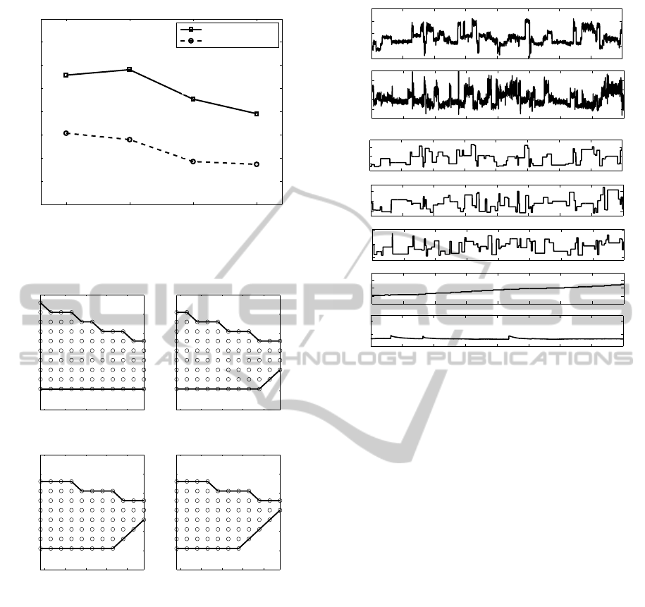
DOE model are shown in Table 2. The feasible HCCI
load range is shown in Figure 1, and the stable HCCI
boundary for different fueling inputs is shown in Fig-
ure 2.
Table 2: Actuator Extremes for stable HCCI (from the
steady state DOE model). The valve events are measured
in degrees after top dead center (deg aTDC).
Input Min Limit Max Limit
Fuel Mass (mg/cyc) 7.0437 12.9161
IVO (deg aTDC) 78 128
EVC (deg aTDC) -119 -69
The A-PRBS sequence is designed to excite the
engine within this stable HCCI region defined by the
DOE model. It should be noted that the DOE filtered
input limits are valid only for steady state conditions
and a large step near the boundary of stable HCCI can
ICINCO2012-9thInternationalConferenceonInformaticsinControl,AutomationandRobotics
388
1500 2000 2500 3000
1
1.5
2
2.5
3
3.5
4
4.5
5
Engine Speed [RPM]
Net Mean Effective Pressure [bar]
Naturally Aspirated Load Range
Upper Load Limit
Lower Load Limit
(2500, 3.27)
(2500, 1.925)
Figure 1: Load range (in NMEP) of naturally aspirated
HCCI engine.
80 90 100 110 120
−130
−120
−110
−100
−90
−80
−70
IVO (deg aTDC)
EVC (deg aTDC)
Fuel Mass − 7.29945 mg/cyc
80 90 100 110 120
−130
−120
−110
−100
−90
−80
−70
IVO (deg aTDC)
EVC (deg aTDC)
Fuel Mass − 7.90625 mg/cyc
80 90 100 110 120
−130
−120
−110
−100
−90
−80
−70
IVO (deg aTDC)
EVC (deg aTDC)
Fuel Mass − 8.59449 mg/cyc
80 90 100 110 120
−130
−120
−110
−100
−90
−80
−70
IVO (deg aTDC)
EVC (deg aTDC)
Fuel Mass − 9.33501 mg/cyc
Figure 2: Stable HCCI operating region at given actuator
settings of IVO, EVC and Fueling.
lead to instabilities. Hence as a means of precaution
against running the engine in an unstable manner and
to save time during experiments, a simple feedback
was created, which attempts a particular input com-
bination and if found to be unstable, quickly skips to
the next combination in the A-PRBS sequence. As
a first attempt, the CA50 was considered the feed-
back signal. During a small time window, any input
combination that resulted in a CA50 above 21 (found
by observing the CA50 during several misfires) is im-
mediately skipped, and the engine is run on the next
combination in the sequence. Finally, post-processing
was performedon the data to removemisfire and post-
misfire data.
A subset of the bounded input signals and the
1000 1500 2000 2500 3000 3500 4000 4500 5000
2
2.5
3
3.5
4
NMEP
(bar)
1000 1500 2000 2500 3000 3500 4000 4500 5000
−5
0
5
10
15
20
CA50
(deg aTDC)
1000 1500 2000 2500 3000 3500 4000 4500 5000
8
10
12
Fuel Mass
(mg/cyc)
1000 1500 2000 2500 3000 3500 4000 4500 5000
80
100
120
IVO
(deg aTDC)
1000 1500 2000 2500 3000 3500 4000 4500 5000
−120
−100
−80
EVC
(deg aTDC)
1000 1500 2000 2500 3000 3500 4000 4500 5000
80
90
100
Coolant
Temp
(deg C)
1000 1500 2000 2500 3000 3500 4000 4500 5000
60
80
cycles
Intake Air
Temp
(deg C)
Figure 3: A-PRBS input-output sequence.
recorded outputs from the engine are shown in Figure
3. It has to be noted that the engine coolant tempera-
ture and the intake air temperature varies slightly dur-
ing the experiment and their variations are recorded
and considered inputs to the model. Nearly 30000
cycles of data were collected, which corresponds to
about 25 minutes of engine testing. About 30% of the
data were found to be arising from unstable operation
and were removed.
4 SVR TRAINING
This section details the training procedure using the
SVR method described in section 2. The SVR is
coded in Matlab using LIBSVM package (Chang and
Lin, 2011). For each output, the model has four
hyper-parametersnamely the system order (n
u
and n
y
,
assumed to be the same), the cost parameter C, ker-
nel parameter ω and SVR parameter ν. To obtain a
model that generalizes well and captures the right or-
der of dynamics, the above hyper-parameters need to
be optimized based on cross-validation.
4.1 Tuning Hyper-parameters
The data set comprising of (x, y) is divided into a
training set that constitutes 80% of the data while
the remaining 20% is separated out for testing. Fur-
SupportVectorMachinesforIdentificationofHCCICombustionDynamics
389
thermore, the training data is divided into validation
training and validation testing data sets for tuning the
model hyper-parameters. The testing data set is never
seen by the model during the training and validation
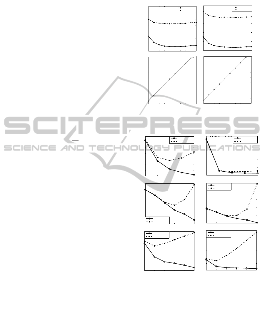
phases. The parameter ν determines the tradeoff be-
tween the spareness and accuracy of the models. An
optimal value of ν results in the minimum model pa-
rameters required for the given accuracy level. It can
be seen using Figure 4 that the knee of the curve
is located at ν of 0.2 and increasing ν beyond this
value doesn’t improve the the prediction accuracy
even though more parameters are used to fit the data
(increase in sparseness). Hence the knee of the valida-
tion error curve is chosen the optimal ν. However for
the case of NMEP, the desired accuracy level has been
achievedwith the minimum value of ν of 0.1. In order
to have a simple model (minimum sparseness), this
value is taken as the optimal ν. In this study, sparse-
ness is defined as follows
sparseness =
n
sv
n
(27)
where n
sv
is the total number of support vectors.
The cost parameter C determines the relative im-
portance given to the outliers and hence the sensitiv-
ity to measurement noise. A large value of C tries to
fit the model for outliers thereby over-fitting the data.
The kernel parameter ω is required to be tuned for
the same reason of having good generalization. The
system order determines the number of previous mea-
surements required to predict the future output. An
optimal value of the order represents the system dy-
namics correctly and a large value not only makes
the model complex by increasing the dimension of
x but also gives a bad prediction of the system’s re-
sponse. It can be seen from Figure 5 that the valida-
tion error increases beyond the optimal values of C,
ω and system order even though training error con-
tinues to decrease. Hence it is important to tune the
hyper-parameters in combination. A full grid search
is performed where the validation training data set
is used to train the model with all combinations of
the considered hyper-parameter values and validation
error found by testing the models on the validation
test data set. Table 3 lists the best combination of
hyper-parametersfor NMEP and CA50 which had the
minimum validation errors. Furthermore the optimal
hyper-parameters are used for retraining with the full
training data set before which it is used for testing.
4.2 SVR Prediction Results
The SVR models with the optimized hyper-
parameters are then trained with the entire training
0.1 0.2 0.3 0.4 0.5 0.6 0.7 0.8 0.9
0.007
0.008
0.009
0.01
0.011
0.012
0.013
0.014
ν
Error
Training Error
Validation Error
0.1 0.2 0.3 0.4 0.5 0.6 0.7 0.8 0.9
0.1
0.2
0.3
0.4
0.5
0.6
0.7
0.8
0.9
1
ν
Sparsity
0.1 0.2 0.3 0.4 0.5 0.6 0.7 0.8 0.9
2.5
3
3.5
4
4.5
5
x 10
−3
ν
Error
Training Error
Validation Error
0.1 0.2 0.3 0.4 0.5 0.6 0.7 0.8 0.9
0.1
0.2
0.3
0.4
0.5
0.6
0.7
0.8
0.9
1
ν
Sparsity
CA50
NMEP
Figure 4: Tuning the accuracy vs sparsity tradeoff parame-
ter ν using cross-validation.
10
−2
10
−1
10
0
10
1
10
2
0.006
0.008
0.01
0.012
0.014
0.016
0.018
0.02
C
Error
Training Error
Validation Error
10
−2
10
−1
10
0
10
1
10
2
0
0.01
0.02
0.03
0.04
0.05
C
Error
Training Error
Validation Error
10
−2
10
0
10
2
0
0.005
0.01
0.015
0.02
0.025
ω
Error
Training Error
Validation Error
10
−2
10
0
10
2
0
0.005
0.01
0.015
0.02
0.025
ω
Error
Training Error
Validation Error
0 1 2 3 4 5
0.004
0.006
0.008
0.01
0.012
0.014
0.016
System Order
Error
Training Error
Validation Error
0 1 2 3 4 5
2
4
6
8
10
12
14
x 10
−3
System Order
Error
Training Error
Validation Error
CA50
NMEP
Figure 5: Tuning cost parameter C, kernel parameter ω and
system order using cross-validation.
data set. The models are then simulated with the un-
seen test data and performance of the models are mea-
sured using mean squared error (MSE) given by
MSE =
1
n
n
∑
i=1
(y
i
− ˆy
i
)
2
(28)
Note that the MSE is different from the loss func-
tion (8) used in SVR modeling. The MSE for the
NMEP and CA50 models during training and testing
are given in Table 4.
ICINCO2012-9thInternationalConferenceonInformaticsinControl,AutomationandRobotics
390

Table 3: Optimal combination of model hyper-parameters.
NMEP CA50
C 1 1
ω 1 1
System Order 1 1
ν 0.1 0.2
Table 4: SVR performance.
NMEP CA50
Training MSE 0.0031 0.0085
Testing MSE 0.0042 0.0103
Model Sparseness 0.1261 0.2283
In order to observe the multi-step-ahead predic-
tions, a completely separate data set is used from
which only the inputs are given to the model along
with the initial conditions of the outputs (delay ini-
tial conditions). Figure 6 and Figure 7 show the pre-
dictions of NMEP by SVR model compared against
the engine’s measured NMEP. Figure 8 and Figure 9
show the predictions of CA50 by SVR model com-
pared against the engine’s measured CA50. It can
be observed that the model predictions match with
the engine’s actual response. It should be noted that
the model’s predictions are based on computer com-
manded step input sequences. The wiggly behavior
in the model’s predictions are due to the variations
in the intake air temperature measurements which are
uncontrollable parameters. HCCI combustion is very
sensitive to the intake air temperature which can be
considered as an independent control input. However
practical realization of such a control system can be
difficult in automotive applications and hence consid-
ered only as a disturbance in the identification model-
ing. It can also be observed that both the steady state
values and the transients are sufficiently captured by
the models except for some regions where there is a
bias offset owing to poor approximations. Lack of
excitations near such input combinations could be a
reason for the bad predictions of the model.
Model sparseness in Table 4 shows that only a
small fraction of the training data set (1892 parame-
ters for NMEP model and 3425 parameters for CA50
model) is used to represent the model efficiently and
these data observations constitute the support vectors
in this method.
5 CONCLUSIONS AND FUTURE
WORK
Support Vector Machines are one of the state of the art
methods for nonlinear regression and the application
0 20 40 60 80 100 120 140 160 180
2.5
3
3.5
NMEP
(bar)
Actual Response
SVR Prediction
0 20 40 60 80 100 120 140 160 180
80
90
100
110
IVO
(deg aTDC)
0 20 40 60 80 100 120 140 160 180
−110
−100
−90
EVC
(deg aTDC)
0 20 40 60 80 100 120 140 160 180
96.5
97
97.5
98
98.5
Coolant Temp
(deg C)
0 20 40 60 80 100 120 140 160 180
52
53
54
Intake Air Temp
(deg C)
Cycles
0 20 40 60 80 100 120 140 160 180
8
10
12
Fuel Mass
(mg/cyc)
Figure 6: Comparison of NMEP (engine output and SVR
prediction).
0 20 40 60 80 100 120 140 160 180
2.6
2.8
3
3.2
NMEP
(bar)
Actual Response
SVR Prediction
0 20 40 60 80 100 120 140 160 180
100
110
120
IVO
(deg aTDC)
0 20 40 60 80 100 120 140 160 180
−115
−110
−105
−100
−95
EVC
(deg aTDC)
0 20 40 60 80 100 120 140 160 180
97
98
99
Coolant Temp
(deg C)
0 20 40 60 80 100 120 140 160 180
51
54
Cycles
Intake Air Temp
(deg C)
0 20 40 60 80 100 120 140 160 180
8
10
12
Fuel Mass
(mg/cyc)
Figure 7: Comparison of NMEP (engine output and SVR
prediction).
of SVR to nonlinear system identification is not abun-
dant in spite of its attractive properties. In this paper a
complex nonlinear dynamic system such as the HCCI
engine is identified using ν-SVR method. Data col-
lection within the stable boundary of HCCI combus-
tion has been accomplished by pre-screening the in-
put sequence using the steady state DOE model of the
engine and by using a closed loop control to avoid un-
SupportVectorMachinesforIdentificationofHCCICombustionDynamics
391

0 20 40 60 80 100 120 140 160 180 200
2
4
6
8
10
12
14
CA50
(deg aTDC)
Actual Response
SVR Prediction
0 20 40 60 80 100 120 140 160 180 200
90
100
110
IVO
(deg aTDC)
0 20 40 60 80 100 120 140 160 180 200
−115
−110
−105
−100
−95
EVC
(deg aTDC)
0 20 40 60 80 100 120 140 160 180 200
96.5
97
97.5
98
98.5
Cooland Temp
(deg C)
0 20 40 60 80 100 120 140 160 180 200
52
53
54
Cycles
Intake Air Temp
(degC)
0 20 40 60 80 100 120 140 160 180 200
8
10
12
Fuel Mass
(mg/cyc)
Figure 8: Comparison of CA50 (engine output and SVR
prediction).
0 20 40 60 80 100 120 140 160 180
0
2
4
6
8
10
12
14
CA50
(deg aTDC)
Actual Response
SVR Prediction
0 20 40 60 80 100 120 140 160 180
100
110
120
IVO
(deg aTDC)
0 20 40 60 80 100 120 140 160 180
−115
−110
−105
−100
−95
EVC
(deg aTDC)
0 20 40 60 80 100 120 140 160 180
97
98
99
Coolant Temp
(deg C)
0 20 40 60 80 100 120 140 160 180
51
52
53
Cycles
Intake Air Temp
(degC)
0 20 40 60 80 100 120 140 160 180
8
10
12
Fuel Mass
(mg/cyc)
Figure 9: Comparison of CA50 (engine output and SVR
prediction).
stable excitations. The dynamics of NMEP and CA50
of naturally aspirated HCCI combustion at constant
speed is modeled using SVR to a good accuracy. Dis-
tinguishing features of ν-SVR including global opti-
mality and sparseness make the method very attrac-
tive compared to traditional neural networks based
identification. Future research would focus on con-
troller development using the SVR models to analyze
the suitability and effectiveness compared to existing
neural network controllers.
ACKNOWLEDGEMENTS
This material is based upon work supported by
the Department of Energy [National Energy Tech-
nology Laboratory] under Award Number(s) DE-
EE0003533. This work is performed as a part of
the ACCESS project consortium (Robert Bosch LLC,
AVL Inc., Emitec Inc.) under the direction of PI
Hakan Yilmaz, Robert Bosch, LLC.
DISCLAIMER
This report was prepared as an account of work spon-
sored by an agency of the United States Government.
Neither the United States Government nor any agency
thereof, nor any of their employees, makes any war-
ranty, express or implied, or assumes any legal liabil-
ity or responsibility for the accuracy, completeness,
or usefulness of any information, apparatus, prod-
uct, or process disclosed, or represents that its use
would not infringe privately owned rights. Reference
herein to any specific commercial product, process,
or service by trade name, trademark, manufacturer,
or otherwise does not necessarily constitute or imply
its endorsement, recommendation, or favoring by the
United States Governmentor any agency thereof. The
views and opinions of authors expressed herein do not
necessarily state or reflect those of the United States
Government or any agency thereof.
REFERENCES
Agashe, S., Ghatol A. and Agashe, S. (2007). Automa-
tion of heat exchanger using neural network. In Inter-
national Journal of Mathematical and Computer Sci-
ences.
Aoyama, T., Hattori Y. Mizuta J. and Sato, Y. (1996). An
experimental study on premixed-charge compression
ignition gasoline engine. In SAE Technical Paper
960081.
Bengtsson, J., Strandh P. Johansson R. Tunestal P. and Jo-
hansson, B. (2006). Model predictive control of ho-
mogeneous charge compression ignition (hcci) engine
dynamics. In 2006 IEEE International Conference on
Control Applications.
Bengtsson, J., Strandh P. Johansson R. Tunestl P. Johans-
son B. (2010). Hybrid control of homogeneous charge
compression ignition (hcci) engine dynamics. In In-
ternational Journal of Control. Taylor & Francis.
ICINCO2012-9thInternationalConferenceonInformaticsinControl,AutomationandRobotics
392

Chang, Chih-Chung and Lin, Chih-Jen (2011). Libsvm: A
library for support vector machines. In ACM Transac-
tions on Intelligent Systems and Technology. Software
available at http://www.csie.ntu.edu.tw/ cjlin/libsvm.
Chiang, C. J. and Chen, C. L. (2010). Constrained control
of homogeneous charge compression ignition (hcci)
engines. In 5th IEEE Conference on Industrial Elec-
tronics and Applications (ICIEA).
Chitralekha, S. B., Shah S. L. (2010). Application of sup-
port vector regression for developing soft sensors for
nonlinear processes. In The Canadian Journal of
Chemical Engineering. Wiley.
Christensen, M., Einewall P. and Johansson, B. (1997). Ho-
mogeneous charge compression ignition (hcci) using
iso-octane, ethanol and natural gas- a comparison to
spark ignition operation. In SAE Technical Paper
972874.
Clarke, S. M., Griebsch J. H. and Simpson, T. W. (2005).
Analysis of support vector regression for approxima-
tion of complex engineering analyses. In Journal of
Mechanical Design.
Drezet, P. M. L. and Harrison, R. F. (1998). Support vector
machines for system identification. In UKACC Inter-
national Conference on Control.
Drucker, H., Burges C. J. C. Kaufman L. Smola A. Vap-
nik V. (1996). Support vector regression machines.
Gretton, A., Douce A. Herbrich R. Rayner P. J. W. and
Scholkop, B. (2001). Support vector regression for
black-box system identification. In Proceedings of the
11th IEEE Signal Processing Workshop on Statistical
Signal Processing.
Hammer, B. and Gersmann, K. (2003). A note on the uni-
versal approximation capability of support vector ma-
chines. In Neural Processing Letters. Kluwer Aca-
demic Publishers.
Hastie, Tibshirani and Friedman (1995). The Elements
of Statistical Learning: Data Mining, Inference, and
Prediction. Springer, 2 edition.
Kim, K. J. (2003). Financial time series forecasting using
support vector machines. In Neurocomputing. Else-
vier.
Kruse, T., Kurz S. and Lang, T. (2010). Modern statistical
modelling and evolutionary optimisation methods for
the broad use in ecu calibration. In 6th IFAC Sympo-
sium Advances in Automotive Control.
Mller, K. R., Smola A. J. Ratsch G. Scholkopf B. Kohlmor-
gen J. and Vapnik, V. (1997). Predicting time series
with support vector machines. In Artificial Neural
Networks ICANN’97. Springer Berlin / Heidelberg.
Ramon, M. M., Alvarez J. L. R. Valls G. C. Mari J. M.
Vazquez A. N. Olivas E. S. Vidal A. R. F. (2006). Sup-
port vector machines for nonlinear kernel arma system
identification. In IEEE Transactions on Neural Net-
works.
Ravi, N., Roelle M. J. Liao H. H. Jungkunz A. F. Chang
C. F. Park S. and Gerdes, J. C. (2009). Model-based
control of hcci engines using exhaust recompression.
In IEEE Transactions on Control Systems Technology.
Schlkopf, B., Bartlett P. Smola A. and Williamson, R.
(1998). Support vector regression with automatic ac-
curacy control. In Proceedings of ICANN’98, Perspec-
tives in Neural Computing.
Schlkopf, B., Smola A. J. Williamson R. C. and Bartlett,
P. L. (2000). New support vector algorithms. In Neu-
ral Computation. MIT Press.
Scholkopf, B. and Smola, A. J. (2001). Learning with Ker-
nels: Support Vector Machines, Regularization, Opti-
mization, and Beyond. MIT Press, Cambridge, MA,
USA.
Smola, A. J. and Schlkopf, B. (2003). A tutorial on sup-
port vector regression. Technical report, Statistics and
Computing.
Sun, J., Zhou Y. Bai Y. and Luo, J. (2006). Nonlin-
ear noise reduction of chaotic time series based on
multi-dimensional recurrent least squares support vec-
tor machines. In Neural Information Processing, Lec-
ture Notes in Computer Science. Springer Berlin / Hei-
delberg.
Thring, R. (1989). Homogeneous-charge compression-
ignition (hcci) engines. In SAE Technical Paper
892068.
Trejo, J. A. R., Yu W. Li X. (2006). Support vector ma-
chine for nonlinear system on-line identification. In
2006 3rd International Conference on Electrical and
Electronics Engineering.
Vapnik, V., Golowich S. E. and Smola, A. (1996). Support
vector method for function approximation, regression
estimation, and signal processing. In Advances in
Neural Information Processing Systems.
Vapnik, V. (1995). The Nature of Statistical Learning The-
ory. Springer, New York.
Wang, X., Du Z. Chen J. and Pan, F. (2009). Dynamic mod-
eling of biotechnical process based on online support
vector machine. In Journal of Computers. Academy
Publisher.
SupportVectorMachinesforIdentificationofHCCICombustionDynamics
393
