Autonomously Traversing Obstacles

Metrics for Path Planning of Reconﬁgurable Robots on Rough Terrain

Michael Brunner, Bernd Br

uggemann and Dirk Schulz

Unmanned Systems Group of the Fraunhofer Institute for Communication, Information Processing and Ergonomics FKIE,

Wachtberg, Germany

Keywords:

Metric, Traversability, Obstacle, Rough Terrain, Reconﬁgurable Chassis, Motion Planning, Mobile Robot,

Autonomy.

Abstract:

The ﬁxed chassis design of commonly employed mobile robots restricts their application to fairly ﬂat environ-

ments, as the wheel diameters or the track heights impose hard limits on their mobility. Unstructured outdoor

and urban environments alike comprehend many different invincible obstacles for most of those systems, like

stairs, boulders or rubble. However, there are mobile robots with reconﬁgurable chassis providing a higher

degree of mobility and enabling them to overcome such obstacles. Yet, current planning algorithms rarely ex-

ploit those enhanced capabilities, limiting these systems to the same environments as the ﬁxed chassis robots.

This paper focuses on the metrics used by our motion planner. The employment of a two-stage planning ap-

proach allows us to use different cost functions for the initial path search and the detailed motion planning

step. The purpose of the initial search is to quickly ﬁnd a fast environment-driven path to the goal. Hence,

it uses fast computable heuristics to assess the drivability, i.e. a risk quantiﬁcation and the utmost operation

limits of the robot model. The detailed planning step determines the desired robot conﬁgurations. For this

purpose, we consider the actuator controls, the system’s stability, an estimate of the traction, and the driving

speed in addition to the quantities used in the ﬁrst stage.

We present experiments to illustrate the inﬂuence of the safety weights and real world experiments which

prove the validity and feasibility of the metrics used by our motion planning algorithm.

1 INTRODUCTION

Fixed chassis robot platforms are commonly used to-

day. These platforms are limited to fairly ﬂat areas, as

their design prevents them from traversing structures

with high edges or steep inclinations. Unstructured

outdoor and urban environments alike include many

different invincible obstacles for most of those robotic

systems, like stairs, boulders or debris. However, mo-

bile robot with reconﬁgurable chassis exist. Altering

the system conﬁguration enhances the mobility of the

robot and enables it to traverse a wide variety of ob-

stacles, which would be insuperable otherwise.

To drive a mobile robot across the above men-

tioned obstacles is a challenging task even for a

trained operator. There are many aspects which have

to be considered when driving over obstacles, most of

which can be neglected for 2D navigation on ﬂat ter-

rain. Especially, the stability of the robot is essential

as the robot falls over more easily. Inertia and mo-

mentum are increasingly important when a fast robot

is operated close to its limits. Moreover, varying con-

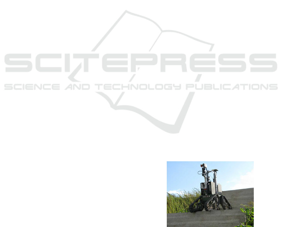
Figure 1: The Telemax robot model, a tracked platform with

four actuators, enabling the system to overcome more com-

plex obstacles than many other robot systems.

tact points of the mobile system change the system’s

behavior to actuator and driving commands.

Introduced planning and controlling algorithms

for traversing rough terrain or overcoming obstacles

depend heavily on the robot’s shape, actuators, and

abilities. This may be comprehensible by considering

that these systems ought to traverse very rough terrain

for which they must operate at their limits. This, in

turn, requires to exhaust the often unique capabilities

Brunner M., Brüeggemann B. and Schulz D..

Autonomously Traversing Obstacles - Metrics for Path Planning of Reconﬁgurable Robots on Rough Terrain.

DOI: 10.5220/0004033400580069

In Proceedings of the 9th International Conference on Informatics in Control, Automation and Robotics (ICINCO-2012), pages 58-69

ISBN: 978-989-8565-22-8

 2012 SCITEPRESS (Science and Technology Publications, Lda.)

given by their speciﬁc actuators. However, more gen-

eral algorithms often apply only to a subset of robots

as the designs of mobile robots differ vastly and use

speciﬁc mechanisms for obstacle traversal.

We developed a two-stage motion planning ap-

proach for reconﬁgurable robots to traverse rough, un-

structured outdoor environments as well as to over-

come obstacles in urban surroundings. We generate a

preliminary path using the platform’s operating limits

instead of the complete robot state and, subsequently,

we apply a detailed motion planning step to reﬁne the

initial path in rough regions. Our algorithm is gen-

eral in the sense that we do not rely on predeﬁned

motion sequences or obstacle classiﬁcations. Further-

more, our algorithm can be used with different robot

models if given a model that can be queried for stabil-

ity.

The metrics used by our motion planner are at the

center of this paper. Many different metrics and cost

functions are proposed for path planning in 2D nav-

igation as well as for rough terrain traversal. Some

quantities, like time or path length, are applicable to

both scenarios. In 2D navigation, aspects like sta-

bility, traction or risk are usually neglected because

they can safely be assumed. In contrast, quantifying

these aspects during planning on rough terrain is es-

sential. In our approach, we use a risk assessment to

adjust the robot’s actions. If performed solely, actua-

tor movements do not increase the path length, thus,

we measure the path execution time to account for

these actions. In rough areas we resort to often em-

ployed quantities, e.g. stability or traction, and incor-

porate them as costs into our approach to determine

appropriate robot conﬁgurations.

The remainder of this paper is structured as fol-

lows: section 2 provides an overview of some related

work. In section 3 we describe the robot model used

for this work. We give a brief scheme of our algo-

rithm in section 4. Section 5 discusses issues of the

sensor coverage for obstacle traversal, the necessity

of global information, and introduces the risk assess-

ment. Sections 6 and 7 illustrate the metrics used for

the initial path search, and the metrics utilized by the

detailed planner in hazardous areas, respectively. We

provide an evaluation of the safety weights and real

world experiments in section 8 and conclude in 9.

2 RELATED WORK

Extensive work has been done on traversability met-

rics and cost functions for path planning of mobile

robots. A binary notion of traversability and the path

length are generally accepted as sufﬁcient measures

in 2D navigation. However, as the terrain becomes

more challenging, more detailed traversability assess-

ments are used and further aspects, like the stability,

the amount of turning, or traction are considered dur-

ing path planning. In this section we outline some of

the previous work done in this area of research.

The National Institute of Standards and Technol-

ogy (NIST) has introduced stepﬁelds as a means of

repeatable test methods for robot mobility to capture

statistically signiﬁcant performance information (Ja-

coff et al., 2008). The NIST also proposed three met-

rics for stepﬁelds; two concerning the coverability of

the terrain, i.e a difﬁculty measure of the entire re-

gion, and one called crossability which depicts the

difﬁculty to move between two speciﬁed locations.

While the coverability is based on the variations in

height difference, the crossability is given by the least

cost path in terms of the terrain roughness along the

path, the amount of turning and the path length. All

metrics are scaled by the robot size and wheel diam-

eter or track height since these parameters inﬂuence

the ability of the robot to overcome obstacles (Molino

et al., 2007). The NIST’s crossability metric is based

on (Iagnemma and Dubowsky, 2004) where the same

quantities are used to include the robot model into

the traversability measure. Since we intent to use the

traversability measure to guide our search algorithm,

a global deﬁnition like the coverability is not suitable.

Similarly, we consider roughness, the amount of turn-

ing and the path length for planning. In contrast, since

the robot size and wheel or track height are not ﬁx for

robots with reconﬁgurable chassis, we do not include

these parameters. Further, we measure the execution

time of a path rather than the path length to account

for actuator movements which do not inﬂuence the

path length, but require time.

In the area of planetary rovers most of the pro-

posed traversability concepts are heavily based on ter-

rain, robot and dynamic models to capture the terrain-

vehicle interactions in detail (Howard and Kelly,

2007). Mechanical models are used to identify the

cohesion and internal friction angles of the terrain

in order to quantify traversability (Iagnemma et al.,

2004). The Traversability Index is a fuzzy rule-based

measure quantifying the slope of the terrain and the

roughness with respect to the size and density of rocks

within the camera frame (Seraji, 1999). It was ex-

tended in (Howard et al., 2001), additionally incorpo-

rating the terrain discontinuity (i.e. cliffs) and hard-

ness as it affects traction. In our approach we also

incorporate an estimate of the vehicle traction, how-

ever, it is less model based.

Many different stability margins were proposed

for measuring the stability of a mobile robot. A

AutonomouslyTraversingObstacles-MetricsforPathPlanningofReconfigurableRobotsonRoughTerrain

comparative overview can be found in (Garcia et al.,

2002). A common way to measure the static stability

of a system is to project the center of mass onto the

supporting polygon. Other stability margins are more

accurate as they consider the height of the center of

mass. In (Miro et al., 2010) the Force-Angle Stabil-

ity Margin (FASM) is incorporated as slowness value

into the Fast Marching Method (FMM) to favor more

stable paths. As we do not contemplate any forces

at this point we use the Normalized Energy Stability

Margin (NESM) (Hirose et al., 2001), also employed

in (Magid et al., 2008).

Others classify the environment using fuzzy rules

and Markov Random Fields to generate so called be-

havior maps which encode preconditions and costs

for a skill-based traversal algorithm (Dornhege and

Kleiner, 2007). Or they label the terrain through ge-

ometric heuristic rules as ﬂat, vertical, stairs or un-

known along with associated costs (penalizing steep

slopes and rough terrain) to apply speciﬁc motion

primitive planners for each class (Rusu et al., 2009).

However, we do not want to base our motion plan-

ning algorithm on a structure classiﬁcation scheme as

this will limit the algorithm to the set of deﬁned struc-

tures. Hence, our metrics solely use general proper-

ties, rather than semantic structure labels.

3 ROBOT PLATFORM

We use a Telerob Telemax robot model in our re-

search, see ﬁgure 1. The robot is 60cm long, 40 cm

wide, and weighs about 70kg. It has 4 tracks which

can be rotated 170

◦

from entirely hinged all the way

down lifting the robot about 45 cm up. Completely

stretched the robot has a length of 120 cm. The robot

is equipped with a skid-drive, and its maximal trans-

lational speed is 1.2

4 BRIEF ALGORITHM

OVERVIEW

In this section we give a short overview of our algo-

rithm. We employ a two-stage planning algorithm for

reconﬁgurable robots to traverse rough environments

and to overcome obstacles in urban areas. Given a

map we ﬁrst compute the risk distribution (section

5) and build a motion graph according to the robot’s

operating limits (section 6). We perform a Dijkstra

search to ﬁnd the initial path in this motion graph.

Afterwards, we identify the path segments leading

through rough terrain and construct a state graph for a

tube-like area around each rough path segment (sec-

tion 7). Using a Dijkstra search we ﬁnd sequences of

robot states including the desired actuator positions.

Finally, applying a default conﬁguration for segments

in ﬂat areas, all segment paths are combined to pro-

vide the ﬁnal path.

5 MAP AND RISK

DISTRIBUTION

Whether a given structure is traversable or not, is not

easily determined. In 2D navigation, this is usually

handled with a simple threshold on the height differ-

ences; everything above this threshold is invincible.

When aiming at overcoming structures, this question

becomes very hard to answer. For 2D navigation a 2D

laser range ﬁnder is sufﬁcient to gather the necessary

information about the surroundings. In contrast, us-

ing a 3D sensor for traversing obstacles and navigat-

ing through rough environments is not enough, due to

the still very limited sensor coverage.

First, installing sensors on a mobile robot intro-

duces a very narrow view; second, determining what

will come after successfully climbing onto an obsta-

cle is very difﬁcult when using common sensors; and

third, while traversing an obstacle the robot’s pose

will often orient the sensors in a way that they are un-

able to cover the environment. For example, consider

the traversal of a ﬂight of stairs; the very narrow view

makes it hard to recognize the stairs especially all the

way up, and while on the stairs and close to the top

the sensors cover very few of the ground. This means,

deciding on the traversability of an obstacle based on

local sensor information is very hard. Therefore, we

came to the conclusion that traversing rough terrain

and obstacles cannot be addressed without global in-

formation like a map. Means of how to deduce the

traversability of a greater area from local sensor in-

formation is beyond the scope of this work.

Further, discovering that an obstacle is actually in-

vincible during traversal is an unpleasant situation. In

this case the robot may be on top of an obstacle and

be required to retreat backwards or, worse, since ob-

stacles are generally not traversable from every an-

gle, the robot may be stuck and, thus, unable to move

safely off the obstacle. A map may help reducing

such incidents but certainly cannot account for all sit-

uations, as a map usually is not detailed enough and

physical aspects, like friction coefﬁcients, are gener-

ally unavailable.

Also related to the ﬁrst point, especially for rough

environments it cannot be assumed that a path to a de-

sired goal exists at all. Moreover, a map allows to as-

ICINCO2012-9thInternationalConferenceonInformaticsinControl,AutomationandRobotics

sess the risk of a path and, thus, enables to determine

whether driving through a hazardous area is worth the

risk or circumventing the obstacle with reasonable ad-

ditional costs is more appropriate.

In addition, a map may be used to improve local-

ization by comparing the robot’s actual pose with the

expected pose deduced from the map. However, the

localization and an enhanced controller are subject to

future work.

Using a map for motion planning in rugged en-

vironments introduces another problem. The validity

of the planning is closely related to the level of detail

of the map. However, large detailed maps are rarely

available. This can be addressed by detailed patches

for rough regions and a greater coarse map.

5.1 Risk Distribution

In our approach we use a heightmap to represent the

environment because it is simple to use and sufﬁcient

for our application. In order to assess the difﬁculty

of a position within the map, we use techniques from

image processing to compute a risk distribution of the

map. As indicator how difﬁcult an area of the map

is, we use the height differences between cells. For

a given map cell c(x,y) we determine the maximal

height difference within a window w of size k

× k

around the cell, i.e., we apply a maximum ﬁlter

c(x,y) = max

, j

),(i

, j

)∈w

x,y

{

|c(i

, j

) − c(i

, j

}

with

x,y

{

(i, j) : |x − i| ≤ k

∧ |y − j| ≤ k

}

However, we prevent a distortion of the range of

values through a threshold h

max

, which conveniently

can be set to the robot model’s maximal traversable

height. Further, the values are scaled to [0,1] using

max

. Subsequently, we perform a Gaussian blur on

this grid of height differences to smooth the transi-

tions and, more importantly to propagate the risk, i.e.

inﬂate large heights and sharp edges. The Gaussian

kernel for a two dimensional blur is deﬁned as

G(x,y) =

2πσ

−

Given kernel sizes of k

and k

for both dimen-

sions, this leads to a matrix G ∈ M(k

+1,k

+1) with

elements

G(i, j) =

2πσ

−

i−



j−



where k

/2 and k

/2 indicate integer divisions. For

each cell in the map we convolve this kernel matrix

Figure 2: Risk distributions of two different maps; left of

a real map build by a laser range ﬁnder and right for an

artiﬁcial urban map. The risk of a region is based on the

height differences in this area. The roughness quantiﬁca-

tion is used to control the planning process. The colors are

indicating the degree of risk, ranging from blue for ﬂat re-

gions over green and yellow to red, high risk areas.

with the window of the same size around the cell. As

the height differences directly correspond to the risk

for the system, we call this smoothed grid of maximal

height difference a risk distribution. Figure 2 shows

the ﬁnal risk distribution of some maps.

Note, comparing, for instance, a ﬂight of stairs

to a ramp of the same gradient angle, the stairs pro-

vides less contact points for traversal with a tracked

robot, and turning is much more severe on these dis-

crete contacts. Hence, a ﬂight of stairs should have

a higher risk compared to a ramp of the same gradi-

ent angle. Using the introduced formulation allows

us to distinguish between those two structures in ex-

actly this way. Moreover, using an appropriate win-

dow size allows us to virtually inﬂate the hazardous

areas, which is commonly done in 2D navigation to

keep the robot away from obstacles. In contrast, high

risk areas are avoided by the robot but if required, do

not prohibit traversal. Another beneﬁt is that the com-

putation is simple and highly parallelizable.

We use this risk distribution in both metrics, for

the initial path search as well as for the detailed mo-

tion planning, to adjust the behavior according to the

difﬁculty of the environment.

6 METRICS FOR THE INITIAL

PATH SEARCH

Driving with reconﬁgurable robots on rough terrain

and over obstacles introduces a large search space and

more constraints compared to 2D navigation must be

satisﬁed. Additionally, the robot’s actuators must be

incorporated into the planning process and the quality

of the path must be judged not only by its length but

also by the robot’s stability and traction, the amount

of turning and time required for actuator movements.

We, therefore, employ a ﬁrst path search to quickly

ﬁnd an environment-driven and fast path to the de-

sired goal location. The path is subsequently used to

AutonomouslyTraversingObstacles-MetricsforPathPlanningofReconfigurableRobotsonRoughTerrain

restrict the search space for the second planning phase

which determines the ﬁnal path consisting of the robot

conﬁgurations including the actuator commands.

Our initial path search employs the introduced risk

distribution. This roughness quantiﬁcation is used to

steer the robot away from hazardous areas and to pre-

fer less risky routes. Usually, an environment consists

of fairly ﬂat areas as well as rugged and challenging

parts. In ﬂat areas, the consideration of the robot’s

complete conﬁguration including actuator values is

not necessary. In contrast, it is essential in rough

areas to increase robot safety and ensure successful

traversal. At this planning phase, we do not know

through which parts of the environment the path will

lead, therefore, we omit the complete state during this

planning stage. We rather stick to the utmost operat-

ing limits of the mobile base neglecting the actuators.

These operation limits do include the maximal roll

and pitch angles before tipover as well as the maximal

traversable height. We identify the least restrictive op-

erating limits through the most stable conﬁguration on

ﬂat ground. However, using a greater set of conﬁgu-

rations generally improves the robot states in terms of

stability as more conﬁgurations can compensate for a

greater variety of situations.

We build a motion graph G

= (V

) which

represents the ability of the mobile robot to traverse

the environment. The vertices v

∈ V

model posi-

tions p

of a dense

regular grid. A vertex v is added

to V

if the maximal risk value r within the robot’s

footprint does not exceed some threshold. If the tran-

sition from a position p

to a neighboring position p

does not violate the robot’s limits in terms of inclina-

tion and height differences, the edge e

i j

= (v

) is

included in E

. Examples of motion graphs are given

in ﬁgure 3.

Using the risk distribution, we are able to deﬁne

the required time t

(i j) to move from a position p

a neighboring position p

as a simple function of the

risk. Let d

i j

be the distance between p

and p

, and

let r

i j

= max(r

) be the higher risk of the involved

positions. Then t

is deﬁned as

(i, j) =

i j

max(v

min

,(1 − r

i j

· w

) · v

max

)

, (1)

where v

min

and v

max

are the minimal and maximal for-

ward velocity, respectively. w

∈ [0, 1] is the safety

weight for the initial path search; low values will

diminish the inﬂuence of the risk distribution and,

hence, lead to possibly shorter, yet more risky paths.

The resolution of the grid is usually half the robot size

to avoid the requirement of intermediate validity test. Also,

situations in which solutions are lost due to the discretiza-

tion are few.

Figure 3: Examples of motion graphs for two different

maps; left for a map of a training hill and right for an ar-

tiﬁcial urban map. The motion graphs encode whether the

given robot model is able to traverse the terrain. Areas with

risk values and slopes below a convenient level are green,

areas with higher risk levels and convenient slopes are yel-

low, and areas with higher risk values and higher slopes are

orange.

Whereas, high values increasingly force the robot to

take low risk paths. Note, the less risky the area, the

faster the robot can drive and the shorter the time.

By using a graph based formulation and encoding the

costs in the edge weights, we are able to perform a

Dijkstra search.

The main purpose of this planning phase is to ﬁnd

a path to the goal which can be used to restrict the

search space for the subsequent detailed motion plan-

ner. Therefore, we differentiate between areas with

risk values and slopes below a convenient level, ar-

eas with higher risk levels and convenient slopes, and

areas with higher risk values and higher slopes (see

ﬁgure 3).

We split the path into segments leading through

ﬂat areas with low risk or no environmental slopes and

segments through rough regions with high risks and

slopes. See ﬁgure 4 for examples. For ﬂat segments

the stability of the robot system can be safely assumed

as done in 2D navigation. Further, any robot conﬁgu-

ration may be applied with no or little risk (given the

pose is stable in itself). Therefore, we do not perform

a detailed motion planning of the robot’s actuator con-

ﬁgurations for ﬂat segments. However, rough regions

require an additional planning of the robot’s actuator

controls and the consideration of the stability to en-

sure safety and task completion. This planning phase

and the metrics used are described in more detail in

section 7. In regions with higher risk values but still

convenient slopes we reduce the velocity of the robot.

Distinguishing between ﬂat and rough areas dur-

ing this planning stage allows us to speed up planning

since we are avoiding unnecessary planning in a high

dimensional space for easily accessible parts of the

environment. However, we ensure the stability and

safety of the robot through a detailed planning step for

rough path segments. Disregarding the robot state and

using the operating limits simpliﬁes the traversability

assessment, hence, the initial path search is fast.

ICINCO2012-9thInternationalConferenceonInformaticsinControl,AutomationandRobotics

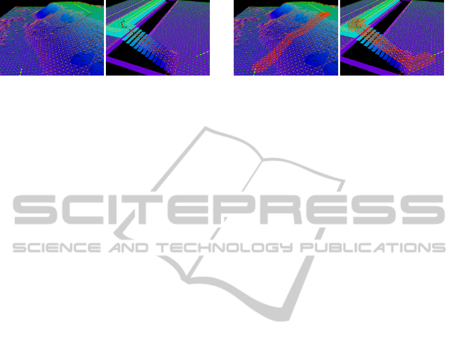
Figure 4: Path segments of the initial paths for two planning

queries on different maps. Segments through ﬂat regions

which do not require further planning are shown in light

green, segments through rough regions will be reﬁned in

the second planning phase and are shown in dark red.

7 METRICS FOR PLANNING IN

ROUGH AREAS

Compared to ﬂat environments, driving on rough ter-

rain is more challenging and exposes the mobile robot

to a greater risk. Therefore, using simply the operat-

ing limits of the robot is not sufﬁcient. We need to

consider the complete robot conﬁguration including

actuator values to estimate the robot’s stability and

traction instead. The conﬁguration of a reconﬁgurable

robot may look like

(x,y, z, θ, ψ,φ,v,ω, ˙v,

ω,a

,...,a

where the ﬁrst part describes the 6D pose of the robot.

The translational and rotational velocities are v and ω,

and the corresponding accelerations are depicted by ˙v

and

ω. a

are the control values of n actuators. The

stability or the contact points with the environment

may also be included in this state. Reducing the state

vector to the controllable part leads to

(x,y, θ, v, ω, ˙v,

ω,a

,...,a

The controllable states still build a large and high

dimensional search space, which cannot be searched

exhaustively. Sample-based methods are usually em-

ployed to handle high dimensional search spaces.

However, sample-based methods provide the ﬁrst

sampled solution, i.e. not necessarily a optimal or

even good. Further, due to their random nature, those

methods struggle to ﬁnd a solution if only a few exist

at all, i.e. they suffer from the narrow passage prob-

lem. Addressing the narrow passage problem and ap-

plying sample-based methods to optimal control is an

active ﬁeld of research. Due to the fundamental is-

sues, we consider sample-based methods as not suited

for solving the problem of traversing rough terrain

and obstacles.

Consequently, we introduce a graph-based ap-

proach using the initial path as basis to restrict the

space of robot states to a tube around this path (see

Figure 5: Two examples of tubes (light red) around the ini-

tial paths in rough areas. The tubes are used to restrict the

search space of the detailed motion planning step.

ﬁgure 5). We, therefore, assume that the best path

with respect to the complete robot conﬁgurations

complies with or is close to the initial path. This as-

sumption mostly holds. It would be violated primarily

if time consuming actuator movements are necessary

by which no distance is gained. This rarely happens

since, ﬁrst, we advocate simultaneous execution of

movements (as described later) and, second, the ini-

tial path prefers less risky routes which generally re-

quire less actuator movements. Finally, the best path

considering the robot’s entire conﬁguration must also

be a fast path.

By using a subsequent planner to reﬁne the path in

rough areas, we are able to apply another cost func-

tion. This, in turn, allows us to increase the impor-

tance of the robot’s safety. The detailed motion plan-

ning accounts for the system’s stability and traction

and for the time consumed by rotation and actuator

movements in order to prevent unnecessary actions.

Since the robot’s speed is very low when traversing

hazardous areas, we neglect forces and dynamic sta-

bility for now. The terms of the cost function for this

planning phase can be divided into a safety term and

a time term.

First, we deﬁne the state graph G

= (V

)

which models a discrete subspace X

⊂ X of the state

space. Each vertex v

∈ V

corresponds to a state

∈ X

. Each edge e

i j

∈ E

models a valid transition

from state x

to x

. The validity of a transition is sub-

ject to the movement constraints of the robot model.

The edge weights are given by the cost function de-

rived in this section. In the following we will use the

state space notation to introduce the metrics.

7.1 System Safety Metric

The safety of the system is affected by several fac-

tors. We incorporate the risk assessment, the system

stability and an estimate of the traction into the safety

metric. To quantify these values we approximate the

robot’s footprint by the best ﬁtting plane using a least-

squares method.

AutonomouslyTraversingObstacles-MetricsforPathPlanningofReconfigurableRobotsonRoughTerrain

Figure 6: Illustration of the Energy Stability Margin. F

and

represent a border of the supporting polygon, i.e. a rota-

tion axis within the plane p. R is the vector from the border

to the center of mass (CM). Θ depicts the angle between R

and the vertical plane and ψ the inclination of the rotation

axis with respect to the horizontal plane. R

is obtained by

rotating R around the rotation axis until it is contained in

plane p. D is computed through D = |R|(1 − cos(Θ)) and

h = |R|(1 − cos(Θ)) · cos(ψ) provides the energy stability

level. Finally, the NESM is deﬁned as s = min

) with

being the normalized energy level of the ith edge of the

supporting polygon.

7.1.1 System Stability

We assess the static stability of the robot using the

Normalized Energy Stability Margin (NESM), see

(Garcia et al., 2002) for a comparative overview of

several stability margins. In contrast to the commonly

used projection of the center of mass onto the support-

ing polygon, the NESM directly provides a notion of

quality.

We will give a short overview of the Normalized

Energy Stability Margin, for a detailed discussion see

(Hirose et al., 2001). The NESM basically indicates

the amount of energy which must be applied to tip the

robot over the “weakest” edge of the supporting poly-

gon. It is derived from the Energy Stability Margin

(ESM) (Messuri, 1985) which is illustrated in ﬁgure

The rotation axis is given by F

and F

as a bor-

der of the supporting polygon within the plane p. R

is the vector from the border to the center of mass

(CM). The angle between R and the vertical plane is

given by Θ, and ψ depicts the inclination of the ro-

tation axis with respect to the horizontal plane. R

obtained by rotating R around the rotation axis un-

til it is contained in plane p. D is computed through

D = |R|(1 − cos(Θ)). Finally,

h = |R|(1 − cos(Θ)) · cos(ψ) (2)

provides the energy stability level for the given rota-

tion axis. The NESM is now deﬁned as

s = min

), (3)

where h

is the normalized energy level with respect

to the ith boundary of the supporting polygon. Our

stability cost is the stability of a robot state x, i.e.

S = 1 − ξ

· s(x), (4)

where ξ

max

is a normalization term using the

maximal stability value of a given robot model to

scale the cost to [0,1].

The computation of the stability of the system de-

pends on the accuracy of the center of mass. There-

fore, we compute the distributed center of mass, as

CM =

∑

i=1

· m

, (5)

where CM is the position of the center of mass of the

system. c

and m

are the centers of mass and the

masses of the n body parts, i.e. the chassis and the

actuators. Thereby, we can determine the center of

mass with respect to the actuator positions which in-

creases the accuracy of the position of the center of

mass.

Due to the minimum function in the stability mar-

gin the stability value may stay the same for several

actuator positions. In order to reach a more stable

conﬁguration the robot might have to perform a se-

quence of actuator movements which do not have an

immediate gain in stability. Therefore, we need an-

other quantity which helps to pass through such se-

quences. We decided to use an estimate of the robot’s

traction.

7.1.2 Traction Estimate

The traction of the robot is increasingly important

when traversing rough terrain or obstacles. However,

we do not want to use any information about the sur-

face properties because maps with information accu-

rate enough to aid planning are very hard to obtain.

Therefore, we estimate the actuators’ ground contact

as an indicator of the traction. The ground contact of

an actuator a

is deﬁned as its angle to the surface.

Then, the traction cost T of a state x ∈ X

is given as

the average over those n angles.

T = ξ

∑

i=1

ψ(a

), (6)

where ψ(a

) is a function providing the angle to the

surface of an actuator a

. ξ

π/2

normalizes the cost

to [0, 1]. Hence, the smaller the angle, the greater the

estimated traction, the safer the robot state in terms of

ICINCO2012-9thInternationalConferenceonInformaticsinControl,AutomationandRobotics

traction. Note, measuring the ground contact of the

actuators in terms of their angle to the surface pro-

vides a qualitative measure of the traction. It can be

viewed as an indicator for traction as the traction be-

tween two objects generally increases with the con-

tact area between those objects. Also, this estimate

serves our purpose of lowering the robot’s actuators

on rough terrain.

The combination of the stability cost, the traction

cost and the risk value of the roughness quantiﬁcation

constitutes the safety term c

safety

of our cost function.

Given two states x

∈ X

the safety cost is deﬁned

safety

(i, j) =

i j

+ T

i j

)

, (7)

where r

i j

= max(r

) is the higher risk of both

states. Similar, S

i j

= max(S

) is the greater stabil-

ity cost of both involved states, and T

i j

= max(T

)

is the maximum traction cost.

7.2 Execution Time Metric

Besides a save path we also want to ﬁnd a fast path to

the goal. In addition, we consider the time required

for rotation and actuator movements which the setup

of the initial path search does not facilitate. For the

initial path search we deﬁned the translational veloc-

ity as a function of the maximum velocity and the

roughness. Since we now have a better understand-

ing of the risk of a robot state, we use the safety cost

safety

of the previous section to adjust the velocity.

(i, j) = ξ

i j

max



min

,(1 − w · c

safety

(i, j)) · v

max



(8)

where d

i j

is the distance between x

and x

, and v

min

and v

max

are the minimal and maximal forward veloc-

ity, respectively. w ∈ [0,1] is the safety weight of the

second planning phase and controls the impact of the

state safety on the planning. This term is also normal-

ized to [0,1] using ξ

max

i, j

The maximal physically possible rotational veloc-

ity depends on the ground contact of the robot’s actu-

ators. For instance, if the actuators of the Telemax

model are completely stretched with a total length

of 1.2m, rotating is practically impossible. We per-

formed several experiments to determine the rota-

tional velocities given the actuator positions and com-

posed a look-up table (for continuous values this

would be a function). Please note, the quantities

are sufﬁcient for planning at this level of detail,

even though they are experimentally established on

ﬂat ground and different surface frictions are ne-

glected. The essential information these values pro-

vide is that the maximum rotational velocity varies

with the robot conﬁguration, and some conﬁgurations

are more qualiﬁed for turning than others. Using this

information the time required for turning from state x

to state x

is given by

= t

(i, j) = ξ

|θ

− θ

(ω(a

) + ω(a

))

, (9)

where θ

and θ

are the orientations of the poses cor-

responding to x

and x

, respectively. ω(·) provides

the rotational velocity of an actuator conﬁguration,

i.e. in our case the value of the look-up table. Fur-

ther, a

= (a

(i),...,a

(i)) is the vector of actuator

controls of x

; a

is deﬁned accordingly. ξ

max

i, j

normalizes the time values to [0,1].

Similar to the previous formulas, we deﬁne the

cost of the actuator movements as the normalized

movement time.

= t

(i, j) = ξ

− a

(i) + v

( j))

, (10)

where a

and a

are deﬁned as before and v

(·) is the

actuator velocity. Again, ξ

max

i, j

scales the val-

ues to [0,1].

To save execution time we would like the system

to perform actions simultaneously. Therefore, the for-

mulation of the time value of our cost function favors

simultaneous execution by implementing the triangle

inequality. We omitted the state variables i and j for

simplicity.

time

(i, j) =

+(1−w·c

safety

)

·t

+(1−w·c

safety

)·t

. (11)

The time value measuring the actuator movements

is scaled by the inverse safety cost since in hazardous

areas and especially in unstable states, we want the

system to apply actuator adjustments which improve

the robot state even if they are time consuming. Note,

this cost function is only applied in rough regions and

may not be applicable in ﬂat areas. In ﬂat areas actu-

ator movements are generally unnecessary and solely

introduce costs, thus, should not be favored.

The cost function used to determine the edge

weights consists of the safety metric and the time

measure. The trade-off between safety and speed can

be adjusted by w ∈ [0, 1] for different mission goals.

Given two neighboring states x

∈ X

the cost of the

transition is deﬁned by

c(i, j) = w · c

safety

(i, j) + (1 − w) · c

time

(i, j). (12)

Note, since all quantities are normalized, the value

of the cost function is also bound to [0,1]. It is im-

portant to state here, that even though we introduced

AutonomouslyTraversingObstacles-MetricsforPathPlanningofReconfigurableRobotsonRoughTerrain

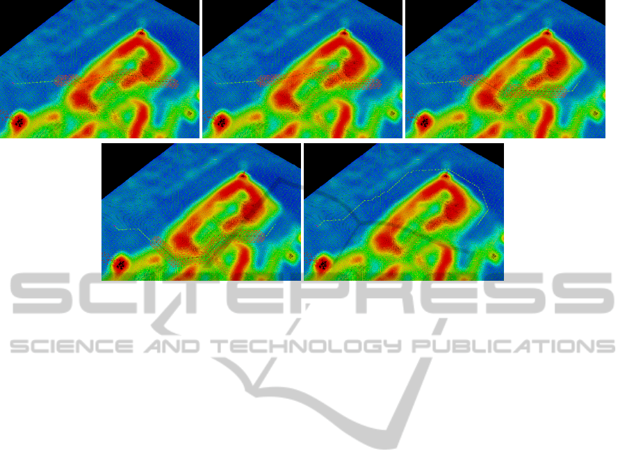
Figure 7: Inﬂuence of the safety weight of the initial path search. It determines the primary direction of the ﬁnal path.

several normalization terms, the only arbitrary values

are the minimal velocity v

min

and the safety weights

and w. All other values are identiﬁed by the robot

model and its abilities. Using a graph-based model

with the deﬁned edge weights allows us to perform

a Dijkstra search on the state graph G

to ﬁnd the

most stable, yet, fastest path to the goal considering

the complete robot state.

8 EXPERIMENTAL RESULTS

In this section we present several experiments. First,

we illustrate the inﬂuence of both safety weights on

the initial path search w

and the detailed motion

planning step w. Second, we preformed tests on real-

world maps with a real robot to prove that our metrics

and plans are valid and executable. To the best of our

knowledge, there are no other approaches which aim

at overcoming arbitrary obstacles with similar recon-

ﬁgurable robots. Hence, we do not provide a com-

parison with other approaches. However, it would be

possible to compare single aspects of our metrics but

we consider this unﬁt to provide any insight of how

well our metrics are suited as a whole for obstacle

traversal compared to others.

8.1 Impact of the Safety Weights

The safety weight of the initial path search w

de-

termines the main direction of the ﬁnal path. Small

weights will lead to short paths, higher values will

cause low risk paths. Figure 7 shows the different

paths obtained for a given start and goal position and

the safety weights 0.0, 0.25, 0.5, 0.75 and 1.0. As

one can see for a weight of 0.0 the path leads to a di-

rect path to the goal position. Increasing the safety

weight forces the algorithm to face the direction of

the steepest gradient when climbing inclinations and

to avoid more and more high risk areas (red). Even-

tually, the path avoids even less risky regions (green)

and circumvents the hill.

While the safety weight of the initial path search

determines the primary course of the ﬁnal path, the

safety weight of the detailed motion planning step w

inﬂuences the driving velocity and the applied actu-

ator conﬁgurations. With an growing importance of

the robot safety the translational velocity decreases

and the changing actuator positions becomes cheaper.

Also, the time required to move the actuators ampli-

ﬁes the execution time. Therefore, with an increasing

safety weight the execution time rises and the safety

cost declines. This trend is shown in ﬁgures 8 and 9.

For these experiments we restricted the detailed mo-

tion planning to the initial path in order to prevent the

path adjustments within the tube to disturb the results

and build a common basis for the comparison.

8.2 Real-world Experiments

We performed tests with the Telerob Telemax model

to prove that the plans proposed by our motion plan-

ner are valid and executable by a real robot. The envi-

ronments are shown in ﬁgures 10 and 12. Both maps

were recorded using a laser range ﬁnder and were sub-

sequently ﬁlled and smoothed to facilitate planning.

Their sizes are 36.4 × 30.45 m and 43.95 × 32.95 m

respectively. For those tests we used the following

ICINCO2012-9thInternationalConferenceonInformaticsinControl,AutomationandRobotics

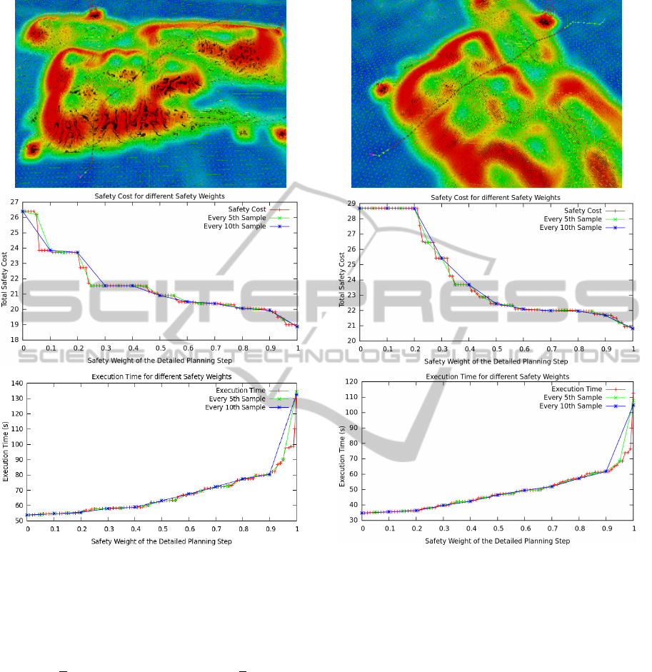
Figure 8: Inﬂuence of the safety weight of the detailed mo-

tion planning step on the execution time and safety of the

path. The top image shows the ﬁrst path used for evalua-

tion.

values: The robot’s maximal traversable height is

max

= 0.5 m. In high risk areas it is allowed to drive

min

= 0.2

and on ﬂat ground v

max

= 1.2

. The dis-

cretization of the maps was 5 cm and the window size

of the ﬁlters is 20 by 20 cells. The resolution of the

motion graph was 30 cm (half the robot length) and we

considered 8 orientations in each point (correspond-

ing to a resolution of 45

◦

). By taking half the robot

length we do not need to perform intermediate valid-

ity tests between two neighboring positions. With re-

spect to the actuator values, both front and both rear

actuators were required to be the same. Further, the

positions were limited to [−45

◦

,45

◦

] in steps of 15

◦

The safety weights were set to w

= 0.75 and w = 0.5.

On the two outdoor environments, we performed

several planning queries of which we present two, one

Figure 9: Inﬂuence of the safety weight of the detailed mo-

tion planning step on the execution time and safety of the

path. The top image shows the second path used for evalu-

ation.

for each map. Figures 11 and 13 show the planned

paths and pictures of the execution by our robot. In

the ﬁrst scenario (ﬁgure 11) the robot had to cross

the hill of rubble through the dips, avoiding the high

risk elevations. The robot was able to follow the pro-

posed path while the planned actuator conﬁgurations

prevented the robot from falling over. Problems dur-

ing the execution where related to the small-grained

material of the rubble which caused the robot to slip

casually. Equally, our robot traversed the hill of the

second scenario given the motion plan shown in ﬁg-

ure 13. The localization was solely based on GPS. In

combination with the inaccuracy of the map made it

difﬁcult for the controller to determine which part of

the plan must be executed.

However, in general, the robot was able to exe-

AutonomouslyTraversingObstacles-MetricsforPathPlanningofReconfigurableRobotsonRoughTerrain

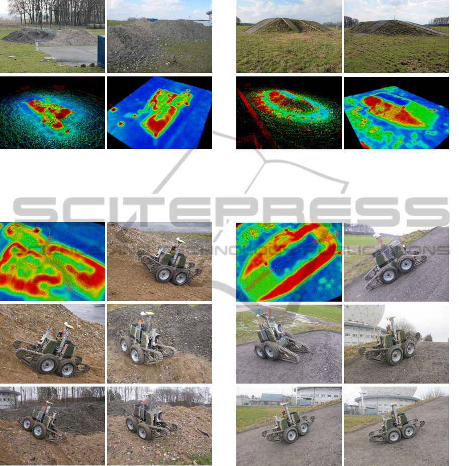
Figure 10: First real-world scenario. The top row shows

two images of the hill of rubble. The bottom row depicts

the point cloud and the ﬁlled, smoothed map. The size of

the map is 36.4 × 30.45 m. The colors indicate the risk of

traversal, ranging from blue for ﬂat regions over green and

yellow to red, high risk areas.

Figure 11: Results of the ﬁrst real-world experiments. The

ﬁrst image depicts the plan given to the robot. The other

pictures show the robot during the execution. If the robot

safety permits, conﬁgurations are sometimes applied in ad-

vanced or while in motion to avoid stop-and-go movement.

cute all plans of our motion planning algorithm and

successfully traversed the obstacles. Further, the pro-

posed conﬁgurations proved to be suited to ensure the

safety of the robot. Problems during the execution

were related to terrain parameters or to inaccuracy of

the sensor data.

Figure 12: Second real-world scenario. The top row shows

two images of the testing hill. In the bottom row the point

cloud and the ﬁlled, smoothed map are depicted. The size

of the map is 43.95 × 32.95 m. The colors indicate the risk

of traversal, ranging from blue for ﬂat regions over green

and yellow to red, high risk areas.

Figure 13: Results of the second real-world experiments.

The ﬁrst image depicts the plan given to the robot. The

other pictures show the robot during the execution. If the

robot safety permits, conﬁgurations are sometimes applied

in advanced or while in motion to avoid stop-and-go move-

ment.

9 CONCLUSIONS AND FUTURE

WORK

In this paper we presented different metrics used by

our motion planning algorithm for robots with recon-

ﬁgurable chassis to ﬁnd paths through rough terrain

ICINCO2012-9thInternationalConferenceonInformaticsinControl,AutomationandRobotics

and over obstacles. By introducing a two-phase plan-

ner we are able to use two different cost functions, one

to ﬁnd a low-risk path to the goal and another suited to

achieve safe robot conﬁgurations along the path. We

introduced a roughness quantiﬁcation which, based

on ﬁltered height differences, provides an estimate

of the risk the robot is exposed to. The presented

cost functions include costs of risk adjusted execu-

tion times and safety parameters, like the stability of

the system and an traction estimate. Using these met-

rics we provided several experiments which prove the

validity of our measures.

As stated in the experiment section, the algorithm

works on a subset of the robot state space X. Im-

proving the state space representation and enhancing

the search method to facilitate a more comprehensive

search for robot conﬁgurations is at the core of our fu-

ture work. Also, we look at the possibilities to over-

come extreme obstacles up to about 40cm in height

as this is the limit given by the manufacturer. This

might require new metrics and a more sophisticated

controller to cope with arising challenges.

REFERENCES

Dornhege, C. and Kleiner, A. (2007). Behavior maps for

online planning of obstacle negotiation and climbing

on rough terrain. In IEEE/RSJ International Confer-

ence on Intelligent Robots and Systems (IROS).

Garcia, E., Estremera, J., and de Santos, P. G. (2002). A

Comparative Study of Stability Margins for Walking

Machines. Robotica, 20:595–606.

Hirose, S., Tsukagoshi, H., and Yoneda, K. (2001). Nor-

malized Energy Stability Margin and its Contour of

Walking Vehicles on Rough Terrain. In IEEE Interna-

tional Conference on Robotics & Automation (ICRA).

Howard, A., Seraji, H., and Tunstel, E. (2001). A rule-

based fuzzy traversability index for mobile robot navi-

gation. In IEEE International Conference on Robotics

and Automation (ICRA).

Howard, T. M. and Kelly, A. (2007). Optimal Rough

Terrain Trajectory Generation for Wheeled Mobile

Robots. International Journal of Robotics Research,

26(2):141–166.

Iagnemma, K. and Dubowsky, S. (2004). Mobile Robots

in Rough Terrain - Estimation, Motion Planning, and

Control with Application to Planetary Rovers, chap-

ter Rough Terrain Motion Planning, pages 51–79.

Springer Tracts in Advanced Robotics.

Iagnemma, K., Kang, S., Shibly, H., and Dubowsky,

S. (2004). Online terrain parameter estimation for

wheeled mobile robots with application to planetary

rovers. IEEE Transactions on Robotics, 20:921 – 927.

Jacoff, A. S., Downs, A. J., Virts, A. M., and Messina, E. R.

(2008). Stepﬁeld Pallets: Repeatable Terrain for Eval-

uating Robot Mobility. In Performance Metrics for

Intelligent Systems (PerMIS) Workshop.

Magid, E., Ozawa, K., Tsubouchi, T., Koyanagi, E., and

Yoshida, T. (2008). Rescue Robot Navigation: Static

Stability Estimation in Random Step Environment. In

Carpin, S., Noda, I., Pagello, E., Reggiani, M., and

von Stryk, O., editors, Simulation, Modeling, and Pro-

gramming for Autonomous Robots, volume 5325 of

Lecture Notes in Computer Science, pages 305–316.

Springer Berlin / Heidelberg.

Messuri, D. A. (1985). Optimization of the locomotion of a

legged vehicle with respect to maneuverability. PhD

thesis, Ohio State University.

Miro, J., Dumonteil, G., Beck, C., and Dissanayake, G.

(2010). A kyno-dynamic metric to plan stable paths

over uneven terrain. In IEEE/RSJ International Con-

ference on Intelligent Robots and Systems (IROS).

Molino, V., Madhavan, R., Messina, E., Downs, A., Bal-

akirsky, S., and Jacoff, A. (2007). Traversability met-

rics for rough terrain applied to repeatable test meth-

ods. In IEEE/RSJ International Conference on Intel-

ligent Robots and Systems (IROS).

Rusu, R. B., Sundaresan, A., Morisset, B., Hauser,

K., Agrawal, M., Latombe, J.-C., and Beetz, M.

(2009). Leaving Flatland: Efﬁcient Real-Time Three-

Dimensional Perception and Motion Planning. Jour-

nal of Field Robotics, 26:841–862.

Seraji, H. (1999). Traversability index: a new concept for

planetary rovers. In IEEE International Conference

on Robotics and Automation (ICRA).

AutonomouslyTraversingObstacles-MetricsforPathPlanningofReconfigurableRobotsonRoughTerrain