
An Integrated Replemishment Model under Dynamic Demand
Conditions
He-Yau Kang
1
, Amy H. I. Lee
2
and Chun-Mei Lai
3
1
Department of Industrial Engineering and Management, National Chin-Yi University of Technology,
Chung-Shan Rd., Taichung, Taiwan, R.O.C.
2
Department of Technology Management, Chung Hua University, Wu-Fu Rd., Hsinchu, Taiwan, R.O.C.
3
Department of Marketing and Logistics Management, Far East University, Zhonghua Rd., Tainan, Taiwan, R.O.C.
Keywords: Lot-sizing, Mixed Integer Programming, Multi-objective Programming, Genetic Algorithm (GA), Safety
Stock.
Abstract: This research develops an integrated replenishment model considering supplier selection, procurement lot-
sizing, quantity discounts and safety stocks under dynamic demand conditions. The objectives of the model
are to minimize total costs, which include ordering cost, purchase cost, transportation cost, shortage cost and
holding cost, and to maximize service level of the system over the planning horizon. First, a multi-objective
programming (MOP) model is proposed in the paper. Next, the model is transformed into a mixed integer
programming (MIP) model based on the
ε
-constraint method. Then, the genetic algorithm (GA) model is
constructed to solve a large-scale optimization problem by finding a near-optimal solution. An example of a
bike manufacturer is used to illustrate the practicality of the proposal model. The results demonstrate that
the proposed model is an effective and accurate tool for the integrated replenishment and logistics
management.
1 INTRODUCTION
Good inventory management is essential for a firm
to be cost competitive and to acquire reasonable
profit in the market. How to achieve an outstanding
inventory management has already been a popular
topic in both the academic field and in real practice.
There are two major categories of inventory models:
deterministic and stochastic.
In deterministic models,
all input data are assumed to be deterministic, and a
mathematical programming model is usually
sufficient to obtain the optimal solution.
For example,
Su and Wong (2008) studied a stochastic dynamic
lost-sizing problem under the bullwhip effect. A
framework of two-stage ant colony optimization
(TACO) was proposed, and a mutation operation
was added in the second stage to determine the
replenishment policy. Stochastic models, on the
other hand, are often limited to highly restricted
assumptions, and most current literature is a
variation of the deterministic lot sizing problem
(Şenyiǧit and Erol, 2010).
The contribution of this research can be
summarized as follows. First, a general formulation
of the lot-sizing problem by mixed integer
programming (MIP) is proposed. The model
considers various costs such as ordering cost,
purchase cost, transportation cost, shortage cost and
holding cost. It aims to minimize the total cost in the
system with safety stock while maximizing the
service level for each planning period. Second, a
genetic algorithm (GA) model is constructed to solve
the problem when it becomes too complicated. We
find that the GA model can find solutions that are
very close to the optimal ones.
The remaining of this paper is organized as
follows. Section 2 reviews some related
methodologies and works. In section 3, the problem
under consideration and the assumptions are
described. The formulation of the lot-sizing problem
by MIP and the construction of the GA model are
presented. Case study is carried out in section 4. In
the last section, some conclusion remarks are made.
614
Kang H., H. I. Lee A. and Lai C..
An Integrated Replemishment Model under Dynamic Demand Conditions.
DOI: 10.5220/0004030706140619
In Proceedings of the 9th International Conference on Informatics in Control, Automation and Robotics (OMDM-2012), pages 614-619
ISBN: 978-989-8565-22-8
Copyright
c
2012 SCITEPRESS (Science and Technology Publications, Lda.)

2 RELATED METHODOLOGY
AND RESEARCH
Dynamic lot-sizing can be referred back to Wagner
and Whitin (1958), and diverse lot-sizing heuristics
have been adopted in many operations management
works.
For example, Teunter, Bayindir and Van Den
Heuvel (2006) studied the dynamic lot sizing
problem for systems with product returns and
remanufacturing, and proposed modifications of the
Silver Meal (SM), least unit cost and part period
balancing heuristics.
Decision makers may want to optimize two or
more objectives simultaneously under various
constraints, and a MOP can then be applied.
A
complete optimal solution seldom exists, and a
Pareto-optimal solution is used then (Wee et al.,
2009).
There are a few methods to derive a
compromise solution (Rosenthal, 1985). For example,
the weighting method assigns priorities to the
objectives and sets aspiration levels for the
objectives. The
ε
-constraint method is a modified
weight method.
One of the objective functions is
optimized while the other objective functions are
incorporated in the constraint part of the model.
GA, a heuristic search process for optimization,
was first developed by Holland (1975). Based on
Darwin’s survival of the fittest principle, GA mimics
the process of natural selection (Maiti et al., 2006). It
has been widely applied to solve production and
operations management problems (Aytug et al.,
2003). The fundamental concept of GA is to code the
decision variables of the problem as a finite length
array, which is called chromosome, and to calculate
the fitness, the objective function, of each string
(Yang, Chan and Kumar, 2012).
3 PROBLEM DESCRIPTION AND
ASSUMPTIONS
The following assumptions and notations are defined
with the modification of those used in the models of
Kang (2008) and Kang and Lee (2010). The
assumptions are summarized as follows:
• The demand of each period is independent and
follows a normal distribution with a constant
coefficient of variation (
θ
).
• At most one order can be placed from each
supplier in each period.
• The replenishment lead time is of known
duration, and the entire order quantity is delivered at
once in the beginning of a period.
• All-units discount schedule is considered. The
price of each unit is dependent on the order quantity.
• The inventory holding cost for each unit is
known and constant, independent of the price of
each unit.
• Planning horizon is finite and known. There are T
periods in the planning horizon, and the duration of
each period is the same.
• The expected ending inventory level in period t
(i.e., the expected beginning inventory level in
period t+1) is the safety stock level in period t.
• The initial inventory level (X
1
) is zero.
All the required notations in this paper are defined
below.
Notations
Indices:
i Supplier (i = 1,2,…, I ).
k Price break (k = 1,2,…, K ).
t Planning period (t = 1,2,…, T ).
v Integer number for calculating the quantity
purchased (v= 1,2,…, V ).
w Integer number for calculating the time
transported (w= 1,2,…, W ).
Parameters:
E(d
t
) Expected demand in period t.
ˆ
t
σ
Standard deviation of demand in period t.
t
σ
Pool standard deviation of demand in period t.
h Inventory holding cost, per unit per period.
r
i
Transportation cost per time from supplier i.
s Shortage cost, per unit per period.
z
α
Standard normal value of service level α.
()Lz
α
Standardized number of units short with
service level α.
M A large number.
o
i
Ordering cost per replenishment from supplier
i.
p
ik
Unit purchase cost from supplier i with price
break k.
q
ik
The upper bound quantity of supplier i with
price break k.
Decision variables:
()
it
PQ Purchase cost for one unit based on the
discount schedule of supplier
i with order quantity
it
Q in period t.
it
Q Purchase quantity from supplier i in period t.
AnIntegratedReplemishmentModelunderDynamicDemandConditions
615

it i
Qb
⎡⎤
⎢⎥
The smallest integer greater than or equal
to
it i
Qb
.
N
it
Number of transportations from supplier i in
period t.
F
it
A binary variable, set equal to 1 if a purchase
is made from supplier i in period t, and 0 if no
purchase is made from supplier i in period t.
X
t
Expected beginning inventory level in period
t.
Y
t
Expected beginning available inventory level
in period t, and
1
I
t t it it
i
YX FQ
=
=+ ×
∑
.
z
t
Standard normal value of ending inventory
level in period t.
()
t
Lz
Standardized number of units short of ending
inventory level in period t
itv
β
A binary variable for calculating the purchase
quantity from supplier i in period t.
itw
G A binary variable for calculating the time of
transportations from supplier i in period t.
itk
U A binary variable, set equal to 1 if a certain
quantity is purchased, and 0 if no purchase is made,
with price break k supplier i in period t.
The above information is used to develop a MIP
model and a GA model to solve the lot-sizing
problem with multiple suppliers and quantity
discounts so that an appropriate inventory level for
each period can be determined. The total cost for
each period can be calculated by adding up the
relevant costs, including ordering cost, holding cost,
and purchase cost with quantity discounts. The total
cost in a planning horizon includes all the total costs
in each period.
3.1 Relevant Costs
The ordering cost for the system is calculated by
equation (1), where o
t
is the ordering cost per time
from supplier i and F
it
represents whether a quantity
is purchased from supplier i in period t.
11
TI
iit
ti
Ordering cost O o F
==
== ×
∑∑
(1)
Equation (2) calculates the purchase cost, where
P(Q
it
) is the unit purchase cost based on the discount
schedule with the order quantity Q
it
, and F
it
represents whether a quantity is purchased from
supplier i in period t.
(( ) )
TI
it it it
t1i1
Purchase cost P P Q Q F
==
== × ×
∑∑
(2)
Equation (3) calculates the transportation cost of the
system, where r
i
is the transportation cost per time
from supplier i,
it i
Qb
⎡
⎤
⎢
⎥
is the smallest integer
greater than or equal to
it i
Qb
from supplier i in
period t, N
it
is number of transportations from
supplier i in period t and b
i
is the maximum
transportation batch size from supplier i.
11 11
TI TI
iiti iit
ti ti
Transportation cost R r Q b r N
== ==
== × = ×
⎡⎤
⎢⎥
∑∑ ∑∑
(3)
The shortage cost of the system is calculated by
equation (4), where s is the shortage cost per unit per
period,
()
t
Lz
is the standardized number of unit
shortage function, and
t
σ
is the pool standard
deviation in period t.
1
()
T
tt
t
Shortage cost S s L z
σ
=
=
=× ×
∑
(4)
The holding cost in period t is equal to the holding
cost per unit times the ending inventory in period t.
Then, the holding cost for a planning horizon is the
summation of the holding cost for each period, as in
equation (5).
1
1
(()
T
tt t
t
H
olding cost H h X L z
σ
+
=
== × +×
∑
(5)
3.2 Multi-objective Programming
(MOP)
The stochastic lot-sizing problem is formulated into
a MOP model for minimizing total cost and
maximizing service level. Based on the
ε
-constraint
method, we can set the total cost as an objective and
use the service level as a constraint. The proposed
model is formulated as follows:
Min ()TC x
(6)
s.t.
x
E
∈
(7)
()
Z
xz
α
≥
(8)
where
z
α
is the standard normal value of service
level α.
3.3 Mixed Integer Programming (MIP)
Model
The multi-objective programming (MOP) problem
can be transformed into a MIP model to solve the
multi-period inventory problem and to determine an
appropriate replenishment policy for each period.
The proposed model can be formulated as follows:
ICINCO2012-9thInternationalConferenceonInformaticsinControl,AutomationandRobotics
616

Minimize
11 1 1
() ()
TI I I
iit it itit i it t t
ti i i
TC o F P Q Q F r N s L z
σ
== = =
⎡
=×+××+×+××
⎢
⎣
∑∑ ∑ ∑
()
1
()
ttt
hX Lz
σ
+
+× + ×
⎤
⎦
(9)
s.t.
1
()
tt t
X
YEd
+
=−
, for all t
(10)
1
I
t t it it
i
YX QF
=
=+ ×
∑
, for all t
(11)
it it
QMF≤×
, for all t
(12)
1
1
2
it
V
v
it itv
v
Q
β
−
=
=
∑
, for all i, t
(13)
it it
i
NQb=
⎡⎤
⎢⎥
, for all i, t
(14)
1
1
2
W
w
it itw
w
NG
−
=
=
∑
, for all i, t
(15)
()
()
tt tt
zYEd
σ
=−
, for all t
(16)
t
zz
α
≥
, for all t
(17)
()
ˆ
tt
Ed
σθ
=×
, for all t
(18)
2
'
'1
ˆ
t
tt
t
σ
σ
=
=
∑
, for all t
(19)
1
()
K
it ik itk
k
PQ p U
=
=×
∑
, for all i, t
(20)
1
(1) (1)
ik itk it ik itk
qMU QqM U
−
+× −≤ <+×−
, for all i, t, k
(21)
1
1
K
itk
k
U
=
=
∑
, for all i, t
(22)
{}
0,1
it
F ∈
, for all i, t
(23)
{}
0,1
itw
G ∈
, for all i, t,w
(24)
{}
0,1
itv
β
∈
, for all i, t, v
(25)
{}
0,1
itk
U ∈
, for all i, t, k
(26)
and all variables are nonnegative.
3.4 Genetic Algorithm (GA) Model
GA is used next to solve the lot-sizing problem with
quantity discounts and safety stock so that near-
optimal solutions can be produced in a short period
of computation time. The procedures of the GA are
proposed as follows:
Step 1. Coding scheme
Assume that at most one order can be placed in each
period and that a replenishment quantity can serve
for an integer number of periods.
Step 2. Initial population of chromosomes
The initial population is generated randomly, and
there are two types of chromosomes, which are also
determined randomly.
Step 3. Fitness function
The fitness function for each chromosome is Min
TC, where TC is the total cost. Min TC is the
minimum cost among all the chromosomes across
the population.
Step 4. Crossover operation
The standard two-cut-point crossover operator is
applied to the selected pair of parent-individuals by
recombining their genetic codes and producing two
offspring.
Step 5. Mutation operator
A mutation operator is to counteract premature
convergence and to maintain enough diversity in the
population. It is performed by changing a randomly
selected gene in the genetic code (0-1, 1-0). In each
generation, all individuals have a set of given genes
fixed, called frozen genes.
Step 6. Selection of subsequent population
After the mutation and crossover operations in each
generation, a subsequent population is selected for
the next generation.
Step 7. Termination
The processes of crossover, selection and
replacement are repeated until the objective function
of the problem is optimized or the stop criterion is
met.
4 CASE STUDY OF A BIKE
MANUFACTURER
4.1 Stochastic Lot-sizing Problem
A stochastic lot-sizing problem with quantity
discounts and safety stock is solved here. Based on
an interview with the management of a bike
manufacturer in Taiwan, the following assumptions
are made. The ordering cost of supplier A (
o
1
) and
supplier B (
o
2
) per replenishment is set to be $220
and $190, respectively. In addition, we set unit
holding cost per period (
h), which includes the
handling cost, storage cost and capital cost, to be
$0.1. The demand in each period is assumed to be
normal distributed with a mean
()
t
Ed and a
coefficient of variation (
θ
) of 1/3. Table 1 shows
the expected demand
()
t
Ed and its standard
deviation
ˆ
t
σ
in each period t.
AnIntegratedReplemishmentModelunderDynamicDemandConditions
617
The ordering cost per time from supplier A and B
is $220 and $190, respectively. The transportation
cost per time is $21 and $20.5 from supplier A and B,
respectively. The unit shortage cost is $30, required
service level is 95%, and the number of periods is 7.
A quantity can be purchased from supplier A and/or
B using the discount schedules in Table 2 and Table
3, respectively.
Table 1: Demand of each period in a planning horizon.
t 1 2 3 4 5 6 7
()
t
Ed
660 700 560 120 650 510 525
Standard
deviation
(
ˆ
t
σ
)
220 233 187 40 217 170 175
Table 2: Discount schedule for supplier A.
Price break (k)
Purchase quantity (q
1k
)
Price per unit
( p
1
k
)
1 0 – 999 $4.00
2 1000 – 1999 $3.92
3 2000 – 2999 $3.84
4 3000 or more $3.76
Table 3: Discount schedule for supplier B.
Price break (k) Purchase quantity
(q
2k
)
Price per unit
( p
2k
)
1 0 – 1500 $4.02
2 1501 – 3000 $3.89
3 3001 or more $3.75
4.2 Experimental Results
The lot-sizing problem is solved by both the MIP
model and the GA model. The MIP model is
implemented using the software LINGO (2006), and
the GA is implemented using the software
MATLAB (2007).
The solution of the MIP model is shown in Table
4.
Under the MIP model, two purchases are made:
3034 units from supplier B in period 1, 1507 units
from supplier B in period 5.
The total cost is $18983.
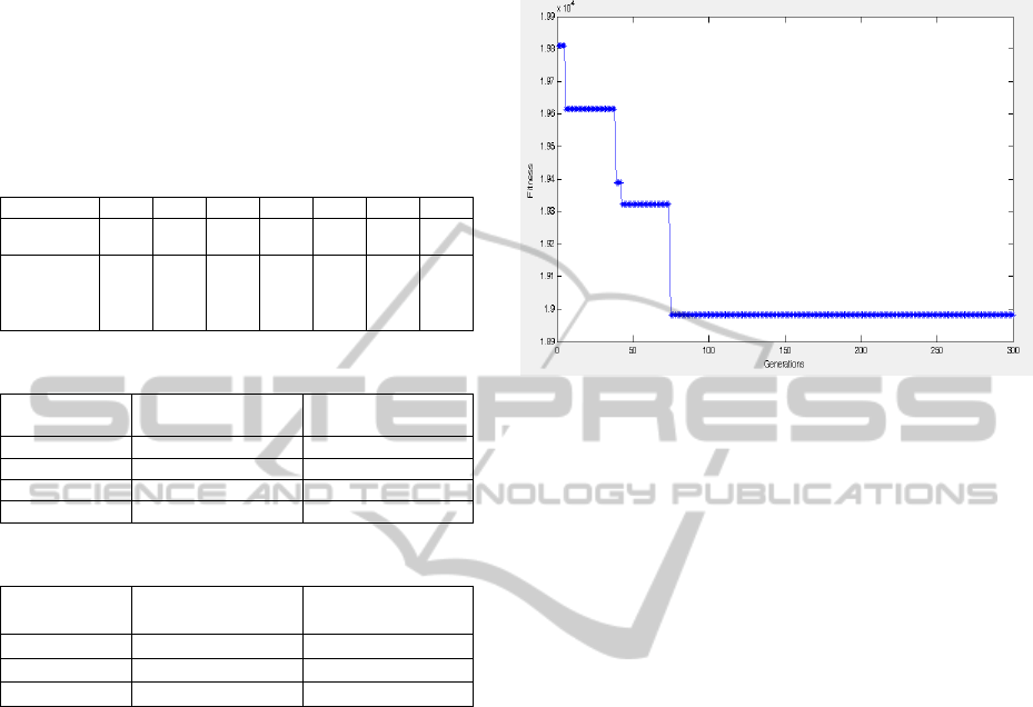
The GA model is implemented by using the
software MATLAB. Two-cut-point crossover for
crossover operations is applied, and an inversion
mutation operator is used to avoid a solution being
trapped in a local optimum and to approach the
global optimum. The size of the initial population is
set as 35. The crossover rate is set as 0.75, meaning
that around 75% pairs of individuals take part in the
production of offspring. The mutation rate is set as
0.01, meaning that each gene of a newly created
solution is mutated with the probability 0.01. The
solutions of the case obtained by the MIP model and
by the GA algorithm are the same, and the total cost
is $18983.
Figure 1: The convergence of GA.
5 CONCLUSIONS
This paper constructs a lot-sizing model with
quantity discounts and safety stock to minimize total
cost over the planning horizon.
A general
formulation of the lot-sizing problem is proposed by
mixed integer programming (MIP) first to devise
appropriate replenishment policies.
An efficient
genetic algorithm (GA) is introduced next for
solving large-scale lot-sizing problem in a very short
time.
Replenishment level and system cost can be
determined after calculating ordering cost, purchase
cost, transportation cost, shortage cost and holding
cost.
The results show that the GA model is effective
in searching for solutions, and it can be very useful
for managers in real practice.
In the future, a more complete case study of
supply chain management can be considered.
A
model that considers issues, such as variable lead
time, probability demand, different priority of
orders, backorder and lost sales, can be developed.
To incorporate these issues, the assumptions will
need to be relaxed by modifying objectives and
constraints.
ACKNOWLEDGEMENTS
This work was supported in part by the National
Science Council in Taiwan under Grant NSC 98-
2410-H-167-008-MY3.
ICINCO2012-9thInternationalConferenceonInformaticsinControl,AutomationandRobotics
618

REFERENCES
Aytug, H., Khouja. M., Vergara, F. E., (2003). Use of
genetic algorithms to solve production and operations
management: a review. International Journal of
Production Research, 41(17), 3955-4009.
Kang, H.-Y., (2008). Optimal replenishment policies for
deteriorating control wafers inventory. International
Journal of Advanced Manufacturing Technology, 35
(8), 736-744.
Kang, H.-Y., Lee, A. H. I., (2010). Inventory
replenishment model using fuzzy multiple objective
programming: A case study of a high-tech company in
Taiwan. Applied Soft Computing, 10, 1108-1118.
LINGO, (2006), LINGO user’s manual, version 10.
Chicago: USA LINGO System Inc.
Maiti, A. K., Bhunia, A. K., Maiti, M., (2006). An
application of real-coded genetic algorithm (RCGA)
for mixed integer non-linear programming in two-
storage multi-item inventory model with discount
policy. Applied Mathematics and Computations, 183,
903-915.
MATLAB, (2007). Using MATLAB, version 7.5.
Massachusetts: The Mathworks.
Rosenthal, R.E., (1985). Concepts theory and techniques:
Principles of multi-objective optimization. Decision
Sciences, 16, 133-152.
Şenyiǧit, E., Erol, R. (2010). New lot sizing heuristics for
demand and price uncertainties with service-level
constraint. International Journal of Production
Research, 48(1), 21-44.
Su, C. T., Wong, J. T. (2008). Design of a replenishment
system for a stochastic dynamic production/forecast
lot-sizing problem under bullwhip effect. Expert
Systems with Applications, 34, 173-180.
Teunter, R. H., Bayindir, Z. P., Van Den Heuvel, W.
(2006). Dynamic lot sizing with product returns and
remanufacturing. International Journal of Production
Research, 44 (20), 4377-4400.
Wagner, H. M., Whitin, T. M., (1958). Dynamic version of
the economic lot size model. Management Science, 5,
89-96.
Wee, H. M., Lo, C. C., Hsu, P. H., (2009). A multi-
objective joint replenishment inventory model of
deteriorated items in a fuzzy environment. European
Journal of Operational Research, 197, 620-631.
Yang, W., Chan, F. T. S, Kumar, V., (2012). Optimizing
replenishment polices using genetic algorithm for
single-warehouse multi-retailer system. Expert
Systems with Applications, 39, 3081-3086.
AnIntegratedReplemishmentModelunderDynamicDemandConditions
619
