
Sigmapoint Approach for Robust Optimization
of Nonlinear Dynamic Systems
Sebastian Recker
1
, Peter K
¨
uhl
2
, Moritz Diehl
3
and Hans Georg Bock
4
1
Aachener Verfahrenstechnik, RWTH Aachen University, Aachen, Germany
2
BASF SE, Ludwigshafen, Germany
3
Optimization in Engineering Center, KU Leuven, Leuven, Belgium
4
Interdisciplinary Center for Scientific Computing, University of Heidelberg, Heidelberg, Germany
Keywords:
Parametric Uncertainty, Optimal Control, Batch Process, Unscented Transformation.
Abstract:
Mathematical models describing dynamic processes contain parametric uncertainties. Robust model-based
optimization thus becomes a challenging task in process engineering. Current approaches either require high
computational effort or they make use of oversimplified approximations that do not capture changes in the
solution structure due to nonlinear effects of the uncertain parameters on the states of the process. In this paper
we propose an improved optimization approach that uses sigmapoints to characterize the space of uncertain
parameters. Propagating sigmapoints through the process model and directly using them in the optimization
problem allows to capture relevant nonlinearities for the uncertain parameters. Main advantages of this simple
yet elegant approach are the relatively low computational burden and the independence from the optimizer, as
no further derivatives are needed. The approach is applied to two examples from process engineering, a batch
distillation and a semibatch reactor.
1 INTRODUCTION
In this paper we consider constrained optimization
problems of the form
min
u∈R
n
u
Φ(x,z,u) (1)
with
Φ :=
Z
T
0
L(x(t),z(t),u(t), p) dt + M(x(T ),z(T ))
(2)
subject to the DAE system
˙x(t) = f (x(t),z(t),u(t), p), t ∈ [0,T ], (3)
0 = g(x(t),z(t), u(t), p), t ∈ [0, T ], (4)
the initial value constraint
x(0) −x
0
= 0, (5)
as well as control and path constraints
h(x(t),z(t),u(t), p) ≤ 0, t ∈ [0,T ]. (6)
In this formulation x(t) ∈ R
n
x
denotes the differential
states, z(t) ∈ R
n
z
the algebraic states, u(t) ∈ R
n
u
the
available controls, and p ∈ R
n
p
the parameters. Such
problems often arise from the model-based optimiza-
tion of technical processes, e.g. in the chemical pro-
cess industry.
The above formulation is based on a process
model with exact parameters p. This is an idealiza-
tion, which is referred to as the nominal problem in
this paper. In most real-world problems, at least some
of the parameters will not be known exactly. Rather,
a set P ⊂R
n
p
that is likely to contain p will be known
or can at least be assumed. For a robust solution of the
optimization problem the constraints shall be fulfilled
for all parameters within this set and thus
h(x(t),z(t), u(t), p) ≤ 0 ∀ p ∈P (7)
has to hold. Due to its then infinite number of con-
straints, this formulation is called a semi-infinite pro-
gram (Blankenship and Falk, 1976). In order to solve
this problem, the number of constraints has to be re-
duced. For this purpose we focus on the general con-
cept of local reduction methods (Hettich and Kor-
tanek, 1993) in this paper. Note that we do not con-
sider the case when the model structure is not entirely
known. In some cases, however, such a problem can
be reformulated into one with parametric uncertainty.
A common idea to solve robust optimization prob-
199
Recker S., Kühl P., Diehl M. and Georg Bock H..
Sigmapoint Approach for Robust Optimization of Nonlinear Dynamic Systems.
DOI: 10.5220/0004026401990207
In Proceedings of the 2nd International Conference on Simulation and Modeling Methodologies, Technologies and Applications (SIMULTECH-2012),
pages 199-207
ISBN: 978-989-8565-20-4
Copyright
c
2012 SCITEPRESS (Science and Technology Publications, Lda.)

lems is to see the uncertain parameters as adverse
players (Ben-Tal and Nemirovski, 1999) that try to
disturb any constraint enforcement effort as strongly
as possible. The task is to still meet the constraints
for the worst parameter realization. This leads to min-
imizing the maximum negative effect of possible un-
certainty realizations with respect to the constraints
and results in the worst-case problem
min
u∈U
Φ(x,z,u, p) (8)
s.t. max
p∈P
h(x,z,u, p) ≤ 0.
Due to its bi-level structure, this optimization prob-
lem is still difficult to solve numerically for general
nonlinear functions.
1.1 Min-max Approximative Worst-case
Reformulation
(Diehl et al., 2006) suggest an approximation for this
kind of optimization problem. If the constraint func-
tions are monotone within the parameter set and can
be approximated by a Taylor expansion, the max-
term of the optimization problem (8) for normally dis-
tributed parameters
P :=
p ∈ R
n
p
|
1
γ
Σ
−
1
2
(p − ˜p)
2
≤ 1
(9)
with the covariance matrix Σ and the confidence level
γ can be restated as:
max
p∈P
h(x,z,u, p)
≈ h(x,z,u, ˜p) + γ
Σ
1
2
∇
p
h(x,z,u, ˜p)
2
≤ 0 (10)
This robust optimization problem can efficiently be
solved by dynamic optimization algorithms. For non-
linear DAE systems this linear approximation may
lead to approximation errors and the robust enforce-
ment of constraints will fail. A remedy is to use
higher order approximations. In (Heine et al., 2006)
a second order approximation of the mean and vari-
ance is suggested that can efficiently be computed by
an unscented transformation.
In this article we assume all uncertain parameters to
be normally distributed. Other parameter distribu-
tions can be treated within the same framework. For a
derivation of robust reformulations of the optimiza-
tion problem for different distributions see (Diehl
et al., 2006).
While we focus on robust enforcement of con-
straints, note that the approach also allows to robustly
treat the cost functional Φ(x,z,u, p).
1.2 Min-max Reformulation with
Sufficient Condition
(Moennigmann and Marquardt, 2002) and (Diehl
et al., 2008) present another approach to handle the bi-
level structure of the optimization problem (8). The
inner maximization problem is replaced by its suf-
ficient condition. Due to the additional equations
this extended optimization problem can be difficult to
solve and results in a higher computational effort, but
overcomes the problems associated with the lineariza-
tion approach.
1.3 Chance-constrainted Programming
Another approach to solve optimization problems ro-
bustly, which avoids the bi-level structure caused by
the worst case min-max formulation of the constraint,
is the chance constrained optimization (Arellano-
Garcia et al., 2003). The general constraint (7) is re-
placed by a probability constraint
P
{
h(x,z,u, p) ≤ 0
}
≥ 1 −α. (11)
This approach requires efficient algorithms for realiz-
ing the mapping from the uncertain parameters to the
uncertain constraints. As this mapping only holds for
the actual set of inputs u, it has to be recalculated in
each iteration of the optimization. Even if derivatives
are used to avoid the computation of the mapping in
each iteration (Li et al., 2008), this approach results
in high computational effort.
2 A MODIFIED SIGMAPOINT
APPROACH
The presented approaches either only hold for mildly
nonlinear problems that can be approximated by
linearization, or they result in high computational
time. To combine the low computational effort of
the worst-case approximation with the higher accu-
racy of the other two methods, we modify the usage
of the unscented transformation suggested in (Heine
et al., 2006). Before optimizing, modified constraints
˜
h(x,z,u, p) shall be identified such that satisfying the
new constraints results in satisfying the original con-
straints for all parameters inside the critical subspace
with a desired probability:
˜
h(x,z,u, p) ≤ 0 ⇒P{h(x,z,u, p) ≤ 0} ≥ 1 −α (12)
A possible choice of the modified constraints could
be the principal axis endpoints of the constraint dis-
SIMULTECH2012-2ndInternationalConferenceonSimulationandModelingMethodologies,Technologiesand
Applications
200

tribution, which correspond to the 1 −α interval
1
, if
the constraints are monotone within the parameter set.
For constraints with moderate curvatures, this choice
of the modified constraints results in an approxima-
tion that might allow to meet the original constraints
for all parameters inside the uncertainty ellipsoid with
nearly the desired probability. In order to identify
these endpoints, the mapping of the parameter distri-
bution onto the constraints has to be described.
An appealing method for propagating distribu-
tions through nonlinear models is the Unscented
Transformation ((Julier and Uhlmann, 1996)). By
choosing so called sigmapoints and weights and prop-
agating these sigmapoints through the model, one
can approximate the distribution of the constraints
˜
h(x,z,u, p), if the weighted sigmapoints approximate
the distribution of the parameters. The first two mo-
ments of the constraint distribution (the mean and the
covariance) are matched exactly and the method can
be extended to match additional moments (Julier and
Uhlmann, 1997).
Using these moments, a possible choice of the
modified constraints for normally distributed parame-
ters is
˜
h := h(x,z,u, ˜p) + γ
h(x,z,u, ˜p) −h(x, z, u, p
UT
i
)
2
,
i = 0,...,2n
p
(13)
with the sigmapoints of the Unscented Transforma-
tion
p
UT
0
= ˜p (14)
p
UT
i
= ˜p +
p
Σ
i
,i = 1, . . . , n
p
p
UT
i+n
p
= ˜p −
p
Σ
i
,i = 1, . . . , n
p
,
where
√
Σ
i
is the ith row or column of the matrix
square root of the covariance matrix Σ. ˜p denotes the
set of nominal parameters. As the first two moments
of the distribution are matched exactly, the endpoints
are matched exactly, if the constraints are normally
distributed. For not normally distributed constraints
the endpoints can be mismatched dramatically, as the
first two moments but not the 1−α intervals are prop-
agated.
Applying the Unscented Transformation to in-
dustrial relevant examples has shown, that modified
sigmapoints are a good approximation for the corre-
sponding 1 −α intervals, even for not normally dis-
tributed constraints. Thus, choosing the modified
1
1 −α denotes the probability of values to lie inside the
symmetric confidence interval with less then γ ·σ from the
mean, with σ representing the standard deviation (e.g. for
normal distributions γ = 1 ⇒ 1 −α ≈ 68.3%, γ = 3 ⇒ 1 −
α ≈99.7%).
constraints as
˜
h := h(x,z,u, p
i
) ≤ 0, i = 0,...,2n
p
(15)
results in satisfying the constraints for all parameters
inside the critical subspace with nearly the desired
probability (1 −α), if the modified sigmapoints are
chosen by
p
0
= ˜p (16)
p
i
= ˜p + γ
p
Σ
i
,i = 1, . . . , n
p
p
i+n
p
= ˜p −γ
p
Σ
i
,i = 1, . . . , n
p
.
Hence, the robust optimization problem results in
min
u∈U
Φ(x,z,u, ˜p) (17)
s.t. h(x,z,u, p
i
) ≤ 0, i = 0,...,2n
p
and can easily be solved by a standard dynamic op-
timizer. For normally distributed and monotone con-
straints the 1 −α intervals are mapped exactly. Ap-
plying this approach to industrially relevant examples
has shown that also for non-normally distributed con-
straints the desired probability is nearly achieved.
3 APPLICATION EXAMPLE:
BATCH DISTILLATION
In the following section we will revisit an example
that has already been studied in previous publications
of (Diehl et al., 2006; Diehl et al., 2008). We will
briefly review the optimization method with the lin-
earization of the max-term and compare their results
to our new approach.
The aim of the process sketched in Figure 1 is the
separation of a binary mixture and to obtain distillate
with a purity of at least 99%. In the following we
briefly summarize the process model.
3.1 Process Model
The content of the reboiler M
0
, with x
0
the molar per-
centage of the lighter component, is heated, so that
vapor with and equilibrium composition y(x) and a
constant molar flux V = 100 kmol/h is produced over
all trays. The vapor equilibrium is expressed by the
simple function y(x) :=
x(1+α)
x+α
. Input to the process
is the controlled reflux ratio R and a liquid molar
flux L =
R
1+R
V , which is also assumed to be constant
throughout the column, is fed back into the column.
The remainder of the condensed liquid flux V −L,
with composition x
C
is collected within the distillate
tank with molar holdup M
D
and composition x
D
. For
SigmapointApproachforRobustOptimizationofNonlinearDynamicSystems
201
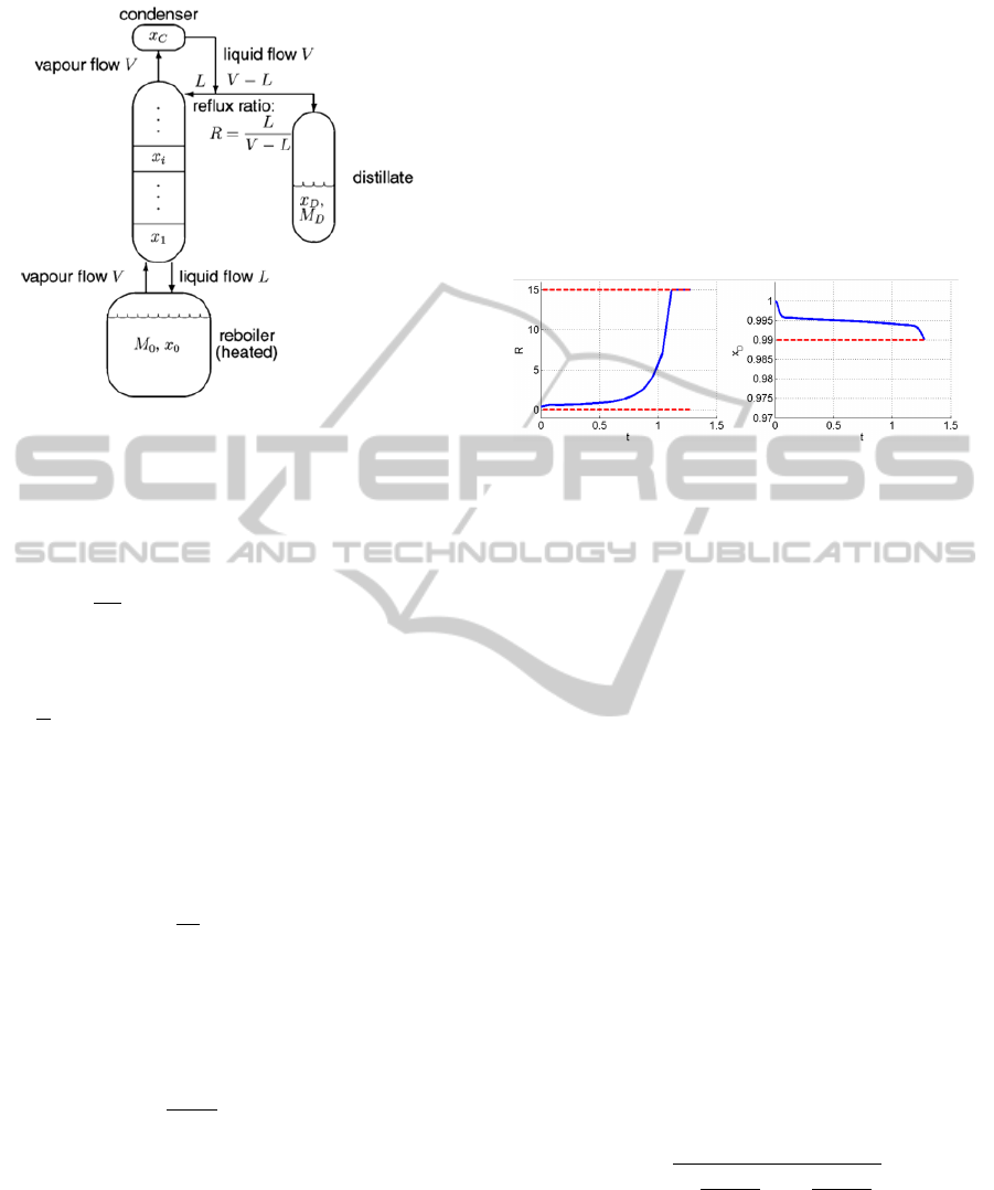
Figure 1: Sketch of the batch distillation column ((Diehl
et al., 2006)).
the reboiler, we get the following ordinary differential
equations:
˙
M
0
= −V + L (18)
˙x
0
=
1
M
0
(Lx
1
−V y(x
0
) + (V −L)x
0
) (19)
and
˙x
i
=
1
m
(Lx
x
i
+1
−V y(x
i
) +V y(x
i−1
) −Lx
i
) i = 1,... ,N
(20)
for the tray concentrations, where m = 0.1 kmol
(the molar holdup of each tray) is assumed to be con-
stant, and the number of trays is N = 5. For the con-
denser concentration x
N+1
we obtain
˙x
N+1
=
V
m
c
(y(x
N
) −x
N+1
) (21)
where m
C
= 0.1kmol is the constant molar holdup of
the condenser, and for the distillate container we ob-
tain
˙
M
D
= V −L (22)
˙x
D
=
V −L
M
D
(x
N+1
−x
D
). (23)
3.2 Nominal Optimization Problem
We summarize the states in x = (M
0
,x
0
,x
1
,...,x
N+1
,
M
D
,x
D
)
T
and set the control variable u = R. The ob-
jective is given by Φ := T −M
D
(T ) and reflects the
two objectives of minimizing the batch time and max-
imizing the produced distillate. The only inequality
constraint is h := 0.99 −x
D
(T ) ≤ 0, i.e. the purity
at the end of the batch shall exceed or equal 99%.
Nominal initial values are M
0
= 100, x
0
= 0.5, x
1
=
... = x
N+1
= x
D
= 1,M
D
= 0.1, and the nominal value
of the equilibrium parameter is α = 0.2. In addi-
tion there are bounds on the controlled reflux ratio,
0 ≤ R ≤ 15. Figure 2 shows the solution for the
nominal optimization problem, which has been solved
with the software package MUSCOD-II ((Leinewe-
ber et al., 2003a; Leineweber et al., 2003b)) based on
the direct multiple shooting approach introduced in
(Bock and Plitt, 1984).
Figure 2: Nominal solution of the batch distillation prob-
lem.
3.3 Uncertain Optimization Problem
For practical problems, the aim of a robust optimiza-
tion is to still meet the constraints despite the un-
certainties. For this model uncertainty is certainly
present in the parameter p
1
= α as well as in the ini-
tial feed composition p
2
= x
0
(0). We assume the set
of the uncertain parameters to be characterized by the
covariance matrix
Σ =
0.0278 0
0 2.5e
−5
. (24)
3.4 Robust Optimization by
Linearization of the Max-term
In order to robustify the optimization with respect to
the critical quality specification, we reformulate the
respective constraint as
max
p∈P
0.99 −x
D
(T, p) ≤ 0 (25)
and approximate the solution of the inner maximiza-
tion problem by
0.99 −x
D
(T, ˜p) −γ
s
Σ
1,1
∂x
D
(T, ˜p)
∂α
2
+ Σ
2,2
∂x
D
(T, ˜p)
∂x
0
(0)
2
≤ 0. (26)
Here, ˜p denotes the nominal parameters and γ is set
to 3, to meet the constraint with aa approximate prob-
ability of ≈ 99.7%. The results for this optimization
are shown in Figure 3.
SIMULTECH2012-2ndInternationalConferenceonSimulationandModelingMethodologies,Technologiesand
Applications
202
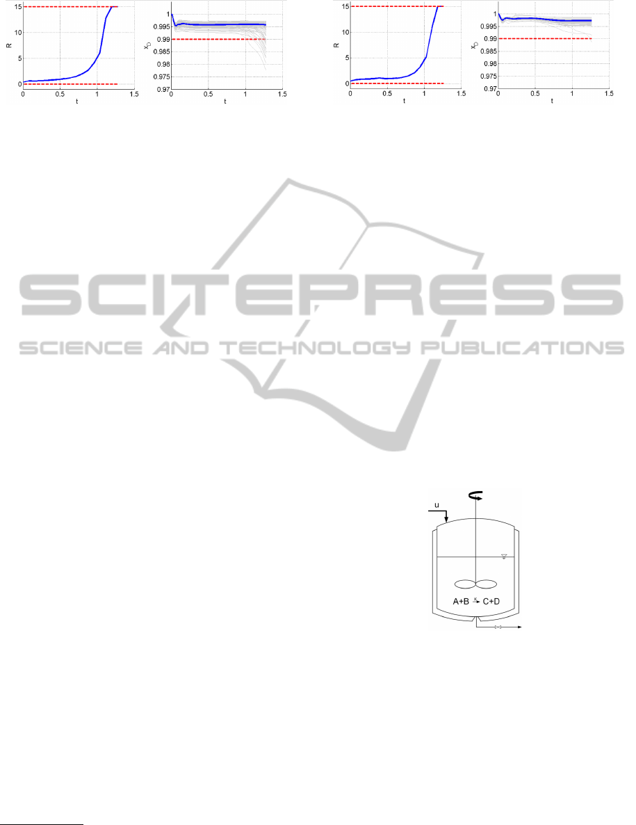
Figure 3: Robust solution of the batch distillation prob-
lem for the linearization of the max-term. Light gray lines
show MonteCarlo simulations with random parameter real-
izations p ∈P .
Although the robust constraint (26) is active, a
MonteCarlo simulation
2
of the robust profile (gray
lines) shows that the desired purity at the end of the
batch is not achieved with the desired probability. Ob-
viously the linearization of the constraint function is
not a sufficient approximation, as shown by (Diehl
et al., 2008). Due to the special properties of this con-
straint function (structural changes of the constraint
function for small changes in the uncertain parameter
x
0
(0)), increasing the order of the Taylor expansion
would not improve the approximation with respect to
the aim of staying above the desired final composi-
tion.
3.5 Robust Optimization by Sigmapoint
Approach
For the sigmapoint approach, the critical constraint
for the nominal parameters ˜p is amended by addi-
tional constraints with the sigmapoints p
i
as argu-
ments. Thus, the robust optimization problem formu-
lation results in
min
u
T −M
D
(T, ˜p) (27)
s.t. 0.99 −x
d
(T, p
0
) ≤ 0
0.99 −x
d
(T, p
1
) ≤ 0
0.99 −x
d
(T, p
2
) ≤ 0
0.99 −x
d
(T, p
3
) ≤ 0
0.99 −x
d
(T, p
4
) ≤ 0
with the sigmapoints (cf. eq. 16)
p
0
= ˜p = (6,0.5)
T
, p
1
= (6.5,0.5)
T
,
p
2
= (6,0.516)
T
, p
3
= (5.5,0.5)
T
, p
4
= (6,0.484)
T
.
The results of the optimization are shown in Fig-
ure 4.
2
For the MonteCarlo simulation the trajectories for 100
normally distributed parameter realizations with mean ˜p
and covariance matrix Σ have been computed.
Figure 4: Robust solution of the batch distillation prob-
lem for the sigmapoint approach. Light gray lines show
MonteCarlo simulations with random parameter realiza-
tions p ∈P .
A MonteCarlo simulation of this profile (gray lines)
shows, that the compliance with the constraint is
achieved with the desired probability.
4 APPLICATION EXAMPLE:
SEMIBATCH PROCESS
The second application example is an exothermic
semibatch process that been considered for optimiza-
tion purposes in a previous publication of (Kuehl
et al., 2005). A sketch of the process is shown in
Figure 5. It describes the esterification of 2-butanol
(B) with propionic anhydride (A) to 2-butyl propi-
onate (D) and propionic acid (C). This homogeneous
reaction is moderately exothermic and is catalyzed by
sulphuric acid (K).
Figure 5: Sketch of the semibatch process.
The reaction is assumed to take place in a semi-batch
reactor under isoperibolic conditions (e.g. constant
jacket temperature). The reactor is initially charged
with B and K. During the process, A is dosed to the
reactor until the dosed amount of substance A is equal
to the initial amount of substance B. The batch is fin-
ished once almost all B has been consumed. A model
of the process can be found in the Appendix. It was
originally developed by (Milewska, 2006).
SigmapointApproachforRobustOptimizationofNonlinearDynamicSystems
203
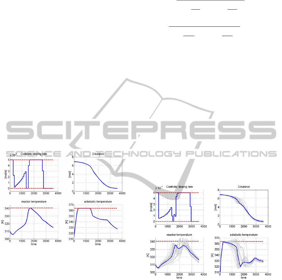
4.1 Nominal Optimization Problem
Following the case study in (Kuehl et al., 2005)
the objective is chosen as Φ :=
R
t
f
0
n
B
(τ)
2
dτ. The
inequality constraints are h
1
(t) := T
R
(t) −340.5 ≤ 0
and h
2
(t) := T
ad
(t) −363.65 ≤ 0.
The complete optimization problem is summa-
rized as
min
u
Z
t
f
0
n
B
(τ)
2
dτ (28)
s.t. 0 mol/s ≤ u(t) ≤ 0.005 mol/s,
Z
t
f
t
0
=0
u(τ) dτ ≤6.89396 mol,
T
R
(t) −340.5 K ≤ 0,
T
ad
(t) −363.65 K ≤ 0.
The second constraint ensures, that the maximum
amount of A is not exceeded. Figure 6 shows the so-
lution of the nominal optimization problem.
Figure 6: Nominal solution of the exothermic semibatch
problem with safety constraints on reactor temperature and
worst-case adiabatic temperature in case of a runaway reac-
tion.
4.2 Uncertain Optimization Problem
Uncertainty is assumed to be present in the jacket
temperature p
1
= T
j
, due to imperfect control action
and in the initial amount of catalyst p
2
= n
K
. The
covariance of the uncertain parameter space is
Σ =
1.2469 0
0 2.8747e
−4
. (29)
4.3 Robust Optimization by
Linearization of the Max-term
To meet the constraints for all p ∈ P the approxima-
tion of the inner worst-case problem reads as
T
R
−γ
s
Σ
1,1
dT
R
dT
j
2
+ Σ
2,2
dT
R
dn
K
2
−340.5 ≤0
(30)
T
ad
−γ
s
Σ
1,1
dT
ad
dT
j
2
+ Σ
2,2
dT
ad
dn
K
2
−363.65 ≤0.
(31)
Figure 7 displays the results for the robust optimiza-
tion for γ = 3. Although this profile results in a safety
margin to the maximal reactor temperature, a Mon-
teCarlo simulation (gray lines) reveals, that the con-
straints are violated more often than allowed.
As the linearization of the uncertain constraints is
computed for each iteration of the optimization, this
approach is suitable for the approximation of uncer-
tainties if the structure of the state trajectories does
not change. This example shows, that even for small
uncertainties (here 1% of the jacket temperatur) the
structure of the trajectories can change dramatically.
This strucutral change caused by the intrinsic dynam-
ics of the system (e.g. accumulation of propionic
acid) is not well approximated by the linearization.
As a consequence, the solution fails to meet the con-
straints for the desired range of uncertain parameter.
Figure 7: Robust solution of the exothermic semibatch
problem for the linearization of the max-term. Light gray
lines show MonteCarlo simulations with random parameter
realizations p ∈P .
4.4 Robust Optimization by Sigmapoint
Approach
As the sigmapoint approach tracks critical points in-
stead of locally approximating the transformed dis-
tribution, the differing trajectories are captured in a
broader range. The robust optimization problem for a
desired probability level of γ = 3 results in
SIMULTECH2012-2ndInternationalConferenceonSimulationandModelingMethodologies,Technologiesand
Applications
204
min
u
Z
t
f
0
n
B
(τ)
2
dτ (32)
s.t. 0 mol/s ≤ u(t) ≤ 0.005 mol/s,
Z
t
f
t
0
=0
u(τ) dτ ≤6.89396 mol,
T
R
(t, p
i
) −340.5 K ≤0, i = 0,...,4
T
ad
(t, p
i
) −363.65 K ≤0, i = 0,...,4
with the sigmapoints (16)
p
0
= ˜p = (313.15,0.0511)
T
, p
1
= (314.65,0.0511)
T
p
2
= (311.65,0.0511)
T
, p
3
= (313.15,0.0562)
T
p
4
= (313.15,0.046)
T
.
The optimization results are shown in Figure 8.
In contrast to the robust solution presented above,
even for the trajectories of the MonteCarlo simula-
tion
3
(grey lines) compliance with the constraints is
achieved with higher probability.
Figure 8: Robust solution of exothermic semibatch prob-
lem for the sigmapoint approach. Light gray lines show
MonteCarlo simulations with random parameter realiza-
tions p ∈P .
5 CONCLUSIONS AND
OUTLOOK
An improved approach for the approximative solu-
tion of robust optimization problems with paramet-
ric uncertainties has been introduced in this paper.
The simple but effective idea relies on propagating
3
To guarantee the comparability for both MonteCarlo
simulations even for the small number (25) of realizations
used in this example, both simulations use the same set of
normally distributed parameters for the trajectories.
sigmapoints through the nonlinear process and ensur-
ing that these sigmapoint trajectories also meet the re-
quired constraints as part of the optimization problem.
This approach does not change the original optimiza-
tion problem apart from adding additional path con-
straints. In particular, no higher-order derivatives are
required. The approach takes advantage of the benefi-
cial properties of the unscented transformation, which
allows to better track the nonlinear effect that uncer-
tain parameters have on the constraints. This proves
particularly important in cases where the structure of
the optimal control problem solution changes. Exam-
ples from process engineering illustrate that even for
small uncertainties these structural changes may oc-
cur and that approaches based on local linearization
of the nominal trajectories may not be well suited.
In practical applications, robustly meeting critical
constraints may not be the only concern. As the ob-
jective function increases with increasing robustness
requirements, one typically wishes to find a compro-
mise between robustness and the costs associated with
it. Within the discussed framework, we see two ap-
proaches to adequately balance robustness and costs.
One solution is to simply price constraint violations
and include these costs in the objective function. The
sigmapoint approach nicely supports this solution as
the requested degree of robustness γ corresponds to
a probability of constraint violation α. We have not
yet investigated whether it is possible to directly in-
clude γ (or α respectively) as a free variable into the
optimization problem.
A second solution for a balanced trade-off be-
tween robustness and performance is a robust refor-
mulation of the objective function itself. For normally
distributed parameters the reformulation of the objec-
tive functions is equivalent to that of 13 seems suit-
able. This has not yet been thoroughly investigated
either.
Even though the sigmapoint approach has per-
formed well on the examples shown, no performance
guarantees have been established so far. There cer-
tainly exist optimization problems where the modified
sigmapoints do not approximate the 1−α interval for
the constraints well enough. In this case a possible
remedy could be the propagation of additional sigma-
points at the expense of higher computational cost.
ACKNOWLEDGEMENTS
The research leading to these results has received
funding from the European Union Seventh Frame-
work Programme FP7/2007-2013 for SYNFLOW and
EMBOCON under grant agreement number NMP2-
SigmapointApproachforRobustOptimizationofNonlinearDynamicSystems
205

LA-2010-246461 and FP7-ICT-2009-4248940.
REFERENCES
Arellano-Garcia, H., Martini, W., Wendt, M., Li, P., and
Wozny, G. (2003). Chance constrained batch distil-
lation process optimization under uncertainty. In IE
Grossmann, CM McDonald (Eds.): Proc. FOCAPO
2003, pages 609–612.
Ben-Tal, A. and Nemirovski, A. (1999). Robust solutions of
uncertain linear programs. Operations Research Let-
ters, 25(1):1–14.
Blankenship, J. and Falk, J. (1976). Infinitely constrained
optimization problems. Journal of Optimization The-
ory and Applications, 19(2):261–281.
Bock, H. and Plitt, K. (1984). A Multiple Shooting algo-
rithm for direct solution of optimal control problems.
In Proceedings of the 9th IFAC World Congress, pages
243–247. Pergamon Press.
Diehl, M., Bock, H., and Kostina, E. (2006). An approx-
imation technique for robust nonlinear optimization.
Mathematical Programming, 107(1):213–230.
Diehl, M., Gerhard, J., Marquardt, W., and Mnnigmann,
M. (2008). Numerical solution approaches for robust
nonlinear optimal control problems. Computers and
Chemical Engineering, 32(6):1287–1300.
Heine, T., Kawohl, M., and King, R. (2006). Robust model
predictive control using the unscented transformation.
In Control Applications CCA, pages 224–230. Perga-
mon Press.
Hettich, R. and Kortanek, K. O. (1993). Semi-Infinite Pro-
gramming: Theory, Methods, and Applications. SIAM
Review, 35(3):380–429.
Julier, S. and Uhlmann, J. (1996). A general method for ap-
proximating nonlinear transformations of probability
distributions. Dept. of Engineering Science, Univer-
sity of Oxford, Tech. Rep.
Julier, S. and Uhlmann, J. (1997). A new extension of
the Kalman filter to nonlinear systems. In Int. Symp.
Aerospace/Defense Sensing, Simul. and Controls, vol-
ume 3, page 26. Citeseer.
Kuehl, P., Milewska, A., Diehl, M., Molga, E., and Bock,
H. (2005). NMPC for runaway-safe fed-batch reac-
tors. In Proc. Int. Workshop on Assessment and Future
Directions of NMPC, pages 467–474.
Leineweber, D., Bauer, I., Bock, H., and Schlder, J. (2003a).
An efficient multiple shooting based reduced SQP
strategy for large-scale dynamic process optimization.
Part 1: theoretical aspects. Computers and chemical
engineering, 27(2):157–166.
Leineweber, D., Schfer, A., Bock, H., and Schlder, J.
(2003b). An efficient multiple shooting based reduced
SQP strategy for large-scale dynamic process opti-
mization. Part II: Software aspects and applications.
Computers and chemical engineering, 27(2):167 –
174.
Li, P., Arellano-Garcia, H., and Wozny, G. (2008). Chance
constrained programming approach to process opti-
mization under uncertainty. Computers & Chemical
Engineering, 32(1-2):25–45.
Milewska, A. (2006). Modelling of batch and semibatch
chemical reactors - safety aspects. Ph.d. thesis, War-
saw University of Technology.
Moennigmann, M. and Marquardt, W. (2002). Normal vec-
tors on manifolds of critical points for parametric ro-
bustness of equilibrium solutions of ODE systems.
Journal of Nonlinear Science, 12(2):85–112.
APPENDIX
The model of the semibatch process (as used in
(Kuehl et al., 2005)) reads as follows:
dn
A
dt
=
u
M
A
−r ·V (33)
dn
B
dt
= −r ·V (34)
dn
C
dt
=r ·V (35)
(C
p,I
+C
p
) ·
dT
R
dt
=r ·(−∆H
r
) ·V −q
dil
−U ·Ω(T
R
−T
J
)
−α ·(T
R
−T
a
) −
u
M
A
·c
p,A
·(T
R
−T
d
)
(36)
where n
i
denotes the molar amount of components
i = A,B,C,D and V the volume. T
R
,T
J
,T
a
and T
d
stand for the reactor, jacket, ambient and dosing tem-
peratures. The reaction rate is denoted by r, (−∆H
r
)
is the reaction enthalpy and Q
dil
the dilution’s heat.
U is an overall heat transfer coefficient and Ω the
heat exchanger area. The approximated heat capac-
ity of solid inserts (stirrer, baffles) is C
p,I
. C
p
denotes
the approximated heat capacity of the entire reaction
mixture and c
p,i
is the specific molar heat capacity of
component i. As the number of moles of D always
equals the number of moles of C, the equation for D
has been omitted. The molar concentrations c
i
are cal-
culated as c
i
= n
i
/V . The molar dosing rate u of A to
the batch reactor serves as control input. The defining
algebraic equations are:
ρ
i
=M
i
P
i
·Q
1−
T
R
T
c,i
0.2857
i
−1
, i = A,B,C,D
(37)
c
i
=
n
i
V
, i = A,B,C,D,K (38)
c
p,i
=a
i
+ b
i
·T
R
+ c
i
·T
2
R
+ d
i
·T
3
R
, i = A,B,C,D
(39)
c
p
=
∑
i=A,B,C,D
c
p,i
·n
i
(40)
SIMULTECH2012-2ndInternationalConferenceonSimulationandModelingMethodologies,Technologiesand
Applications
206
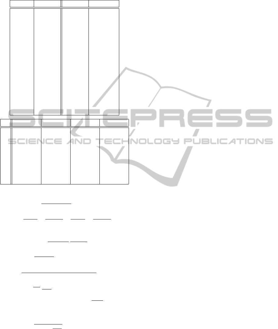
Table 1: List of process parameters and initial conditions.
name value name value
Ω
min
0.0113 n
1
1.58
V
min
0.124 n
2
0.76
d 0.155 E
a
9.17·10
4
V
1
0.8 A
1
9.35·10
10
V
2
1.6 A
2
9.22·10
10
C
p,I1
117.3 A
3
9.78·10
10
C
p,I2
198.4 A
4
1.40·10
8
U
1
195 R 8.314
U
2
155 (−∆H
r
) 59458
α 0.1 T
R
(0) 310
T
J
313.15 n
A
(0) 0.0
T
d
298.15 n
B
(0) 6.894
T
a
298.85 n
C
(0) 0.0
m
A,total
890.00 n
K
0.0511
q
0
1.6 ·10
4
i A B C D
M
i
0.13014 0.07412 0.07408 0.13011
a
i
683.73 242.57 94.84 206.16
b
i
-3.701 -2.313 -0.243 0.199
c
i
9.6·10
−3
1.07·10
−2
2.2·10
−3
-3.56·10
−4
d
i
-7.46·10
−6
-1.16·10
−5
-2.51·10
−6
1.04·10
−6
P
i
0.462 0.320 0.285 0.508
Q
i
0.2166 0.2088 0.1993 0.2265
T
c,i
630 536 611 578
C
p,I
=C
p,I1
+
C
p,I2
−C
p,I1
V
2
−V
1
(V −V
1
) (41)
V =
n
A
M
A
ρ
A
+
n
B
·M
B
ρ
B
+
n
C
M
C
ρ
C
+
n
C
·M
D
ρ
D
(42)
Ω = Ω
min
+ 4 ·
V −V
min
d
1m
3
1000 ·l
(43)
U =U
1
+
U
2
−U
1
V
2
−V
1
(V −V
1
) (44)
x
A
=
n
A
(t)
n
A
(t) + n
B
(t) + 2n
C
(t) + n
K
(0)
(45)
q
dil
=q
0
·e
−x
A
0.14
dn
A
dt
(46)
r =
A
1
+ A
2
·c
n
1
C
(t) + A
3
·c
n
2
K
e
−E
a
R·T
R
(t)
·c
A
·c
B
(47)
T
ad
=T
R
+
n
A
·∆H
900 ·c
p
·V
1000
(48)
In these equations, M
i
, ρ
i
, c
i
denote the molar weight,
density and molar concentration of component i. V
1
,
V
2
, U
1
, U
2
are geometry-dependent parameters and
d is the scaled reactor diameter. The rate of heat
loss to the environment is modeled by a constant α
of appropriate dimension derived from a constant
heat transfer coefficient and an average heat transfer
surface area. The reaction rate is calculated following
an Arrhenius approach; the parameters A
i
and n
i
are
estimated from experimental data and give very good
results for the semi-batch operation mode.
SigmapointApproachforRobustOptimizationofNonlinearDynamicSystems
207
