Predictive Control of Unmanned Formations

Martin Saska and Libor P

reu

cil

Department of Cybernetics, Czech Technical University in Prague, Technick

a 2, Prague, Czech Republic

Keywords:

Mobile Robots, Formation Control, Receding Horizon Control, Obstacle Avoidance.

Abstract:

A receding horizon control based approach for guiding of autonomous formations of nonholonomic robots

in a leader-follower constellation is proposed in this paper. The presented method ensures dynamic obstacle

avoidance, formation coordination as well as failure tolerance. The robustness of the algorithm is veriﬁed by

numerical multi-robot experiments. Besides, effects of system’s parameters on the algorithm performance are

investigated.

1 INTRODUCTION

Formation driving of nonholonomic robots in an envi-

ronment with dynamic obstacles are required in many

robotic applications. As an example, one can mention

airport snow shovelling by formations of snow plows

(Saska et al., 2008) being our target application. In

these tasks, the trajectory planning for the whole for-

mation and the formation maintenance and stabiliza-

tion have to be encapsulated into a complex system

being able of responding to dynamic environment and

unforeseen events.

Plenty of studies investigating formation con-

trol and planning have been published recently, e.g.

(Zhang, 2010; Liu and Jia, 2012). These algorithms

are mostly focused on tasks of formation following a

predeﬁned path and formation stabilization in desired

positions. However, there is a lack of adequate meth-

ods in the literature for providing ﬂexible control in-

puts for members of the formation responding to the

dynamic environment and handling together optimal-

ity and stability of the leader-to-goal and followers-

in-formation tasks. We propose a novel method solv-

ing these challenges.

In the proposed system, the response to unfore-

seen events such as appearing dynamic obstacles or

failures of team members is ensured by Receding

Horizon Control (RHC), which is also known as the

model predictive control. RHC is an optimization

based technique often used for stabilizing linear and

nonlinear dynamic systems. For a detailed survey of

RHC methods we refer to (Mayne et al., 2000) and

references reported therein. The works applying RHC

for the formation driving are presented in (Dunbar

and Murray, 2006; Chen et al., 2010). Algorithms

in these papers have utilized RHC for the formation

stabilization and/or following predeﬁned trajectory in

a workspace without obstacles.

Our contribution is a new concept of RHC that

combines both, the trajectory planning to a goal re-

gion for the entire group and the maintenance and

stabilization of the formation, into one optimization

process via an additional planning horizon. This ap-

proach enables to navigate the formation in such a

way that the local image as well as the overall struc-

ture of the environment are appropriately incorpo-

rated. On top of that, the contribution of this paper

lies in the study of RHC’s parameters on the algo-

rithm performance.

2 METHOD DESCRIPTION

Leader Trajectory Planning and Control. The

main idea of the receding horizon control is to solve

a moving ﬁnite horizon optimal control problem for

a system starting from current state or conﬁguration

ψ(t

) over the time interval [t

] under a set of con-

straints on the system states and control inputs. In

this framework, the length t

− t

of the time inter-

val [t

] is known as the control horizon. As a

result of the optimal control loop, a sequence of N

states of the system (transition points) is found. Be-

tween these points, the control inputs, which navi-

gate the robot from one transition point to the fol-

lowing one, are constant. After a solution from the

optimization problem is obtained on a control hori-

zon, a portion of the computed control actions is ap-

403

Saska M. and P

reu

cil L..

Predictive Control of Unmanned Formations.

DOI: 10.5220/0003994404030406

In Proceedings of the 9th International Conference on Informatics in Control, Automation and Robotics (ICINCO-2012), pages 403-406

ISBN: 978-989-8565-22-8

 2012 SCITEPRESS (Science and Technology Publications, Lda.)

plied on the interval [t

,∆tn+t

], known as the reced-

ing step. This process is then repeated on the inter-

val [t

+ ∆tn,t

+ ∆tn] as the ﬁnite horizon moves by

time steps deﬁned by the sampling time ∆tn, yield-

ing a state feedback control scheme strategy. Advan-

tages of the RHC scheme become evident in terms of

adaptation to unknown events and change of strategy

depending on new goals.

In the presented approach, we propose to solve the

collision free trajectory planning and the optimal con-

trol together in one optimization step. We extend the

standard RHC method with one control horizon into

an approach utilizing two ﬁnite time intervals T

and

. The ﬁrst time interval T

should provide immedi-

ate control inputs for the formation regarding the local

environment. The difference ∆t(k + 1) = t

k+1

−t

be-

tween transition points is kept constant in this time

interval. The second interval T

takes into account

information about the global characteristics of the en-

vironment to navigate the formation to the goal. The

transition points in this part can be distributed irregu-

larly to effectively cover the environment. During the

optimization process, more points are automatically

allocated in the regions where a complicated maneu-

ver of the formation is needed. This is enabled due

to the varying values of time ∆t(k + 1) = t

k+1

−t

be-

tween the transition points. Both these control inter-

vals, T

and T

together form a trajectory Ω from

an actual position of the robot into a desired target

through N + M transition points.

The trajectory planning and the static as well

as dynamic obstacle avoidance problem can be then

transformed to the minimization of a single cost func-

tion J(Ω) subject to sets of constraints. During the op-

timization, both control vectors and transition points

act as variables and can be optimized to get the de-

sired solution. The proposed cost function consists of

three parts as J(Ω) = J

total time

(Ω) + αJ

obst dist

(Ω) +

βJ

deviation

(Ω).

The endeavor of the trajectory planning to reach

a desired goal as soon as possible is expressed in the

ﬁrst part, which represents the total time required for

reaching the goal if using the trajectory Ω. It is a

sum of time differences ∆t(·) between all transition

points of Ω. The second part J

obst dist

(Ω) is an avoid-

ance function, which contributes to the ﬁnal cost if

an obstacle is closer to the trajectory than a certain

detection radius and it approaches inﬁnity if distance

to the closest obstacle is equal to an avoidance radius.

The part J

deviation

(Ω) is employed only if it is required

to follow a preferred path during reaching the target

(as the following of runway axes shown in Fig. 2-5).

This part represents the biggest deviation of a transi-

tion point from the desired path to follow. If the aim

of the planning is to reach the target independently

on a desired path, this part is neglected (as shown in

Fig. 1). The inﬂuence of all parts of the cost function

is adjusted by constants α and β.

The minimization of the cost function is subject

to a set of equality constraints representing a kine-

matic model of the utilized vehicles. This satisﬁes

that the obtained trajectory stays feasible with respect

to kinematics of nonholonomic robots. Besides, it is

subject to a set of inequality constraints that charac-

terizes bounds on the velocity and curvature of the

virtual leader. These bounds are determined by the

shape of the formation and motion constraints of each

of the follower. Finally, a stability constraint guaran-

teeing that the obtained trajectory will enter the target

has to be employed. This inequality constraint rep-

resents distance between the target and the last tran-

sition point of Ω. The constraint is satisﬁed if this

distance is bellow a given threshold.

Trajectory Tracking for the Followers. The pre-

sented approach relies on the well known leader-

follower method (Barfoot and Clark, 2004), where the

followers track the leader’s trajectory, which is dis-

tributed within the group. The followers are main-

tained in relative distance to the leader in curvilinear

coordinates. Employing this concept, the trajectory

computed as the result of the previous section will be

used as an input of the trajectory tracking for the fol-

lowers. We apply the classical RHC based method

with one control interval T

for a discrete-time trajec-

tory tracking. Such a scheme enables to respond to

events in the environment behind the actual position

of the leader and to incorrect movement of a neigh-

bour in the formation. One can ﬁnd implementation

details on this approach in (Saska et al., 2011), where

such a trajectory planning has been used for a spline

path following.

3 EXPERIMENTAL RESULTS

AND PARAMETERS SETTING

Let us now discuss the inﬂuence of parameters n,

N and M and show performance of the method via

numerical experiments and simulations. In Table 1,

where the situation from Fig. 1 was solved, the quality

of results (values of the cost function) and computa-

tional time

are presented. As expected, the quality of

the results increases with growing parameter M, as is

also shown in Fig. 1, but the necessary computational

In the 2nd and higher steps of the planning loop, the

computational time is notably decreased due to possible re-

initialization using the result from the previous step.

ICINCO2012-9thInternationalConferenceonInformaticsinControl,AutomationandRobotics

404

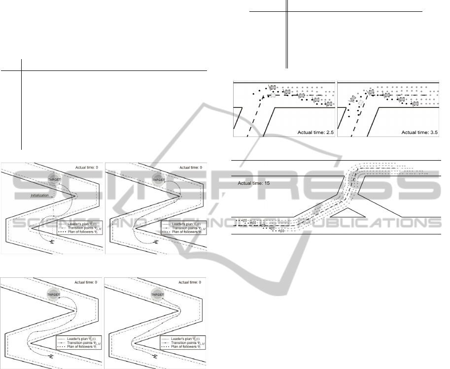
Table 1: Computational times required for planning the ﬁrst

step of the algorithm, the maximal computational times re-

quired for the second and higher steps of planning and val-

ues of the cost function J(Ω) after the ﬁrst step of the al-

gorithm. The algorithm was used with different values of

parameter M and ﬁxed constants N = 4, n = 2. The re-

sults have been obtained with Pentium 4 CPU 3.2GHz using

function fmincon of Matlab.

M t [s] (1.st) t

max

[s] (≥ 2.st) cost [-] (1.st)

2 34.7 0.28 ∞

3 34.9 0.29 38.8

4 43.4 0.36 27.8

5 54.7 0.49 21.1

6 68.4 0.61 15.7

7 82.5 0.75 13.1

8 99.3 0.93 11.6

(a) M = 2. Infeasible path with col-

lisions.

(b) M = 3. Temporary contractions

of shape required.

Figure 1: Solution of the formation to target zone problem

with different setting of parameter M.

time of optimization is increased.

The inﬂuence of parameters n and N will be

demonstrated using the results of the RHC method

applied for driving of formations of autonomous

ploughs at airport with two parallel runways con-

nected via several auxiliary roads (see Fig. 2). The

task of the ploughs is to follow the axes of roads

that need to be cleaned. The crucial problem of the

method is to overcome unsmooth connections of axes

and still to maintain the optimal coverage of the run-

ways. We purposely did not smooth the desired path

in a post-processing to highlight the effect of the vari-

ables n and N.

Now, let us deﬁne an interval of stabilization

IS(T h) to be able to numerically characterise the in-

Table 2: Values of IS(d

/4) of solutions obtained by the

algorithm with a different setting of parameters N and n.

n \\N 2 3 4 6 8

1 ∞ 2.44 2.19 1.50 1.50

2 ∞ 2.35 1.99 1.48 1.44

3 x ∞ 2.44 2.05 1.50

4 x x ∞ 2.16 1.49

5 x x x 2.72 2.69

(a) Response to the path break. (b) The ploughs turn with minimal

turning radius.

trajectories of the ploughs.

Figure 2: Formation driving algorithm with parameters N =

3 and n = 2.

ﬂuence of different setting of variables n and N. The

interval of stabilization IS(T h) will be the length of

the desired path between the connection of line seg-

ments of the desired path and the point from which

the difference between the virtual leader position and

the desired position on the followed path stays less

than or equal to a threshold T h as long as the plan-

ning interval N does not reach the next connection of

line segments.

The values of IS(T h) for Th = d

/4, were d

width of the robot, obtained from simulations of the

task in the Fig. 2 using the RHC method with differ-

ent settings of parameters N and n are presented in

Table 2. The obvious result is the correlation of solu-

tions’ quality with the value of N. Longer time hori-

zon can response to the sudden changes of the forma-

tion heading better. For the lowest values of N the

process can be even unstable (denoted as ∞ in the ta-

ble). Contrariwise a too big value of the parameter n

causes a long period of the formation driving without

any possibility to respond to obstacles or to a break-

age of the desired path.

In Fig. 2, the simulation with setting of algorithm

n = 2 and N = 3 is presented to demonstrate the effect

of the insufﬁciently long time interval N. In all pic-

tures, the black points denote an actual plan for the

PredictiveControlofUnmannedFormations

405

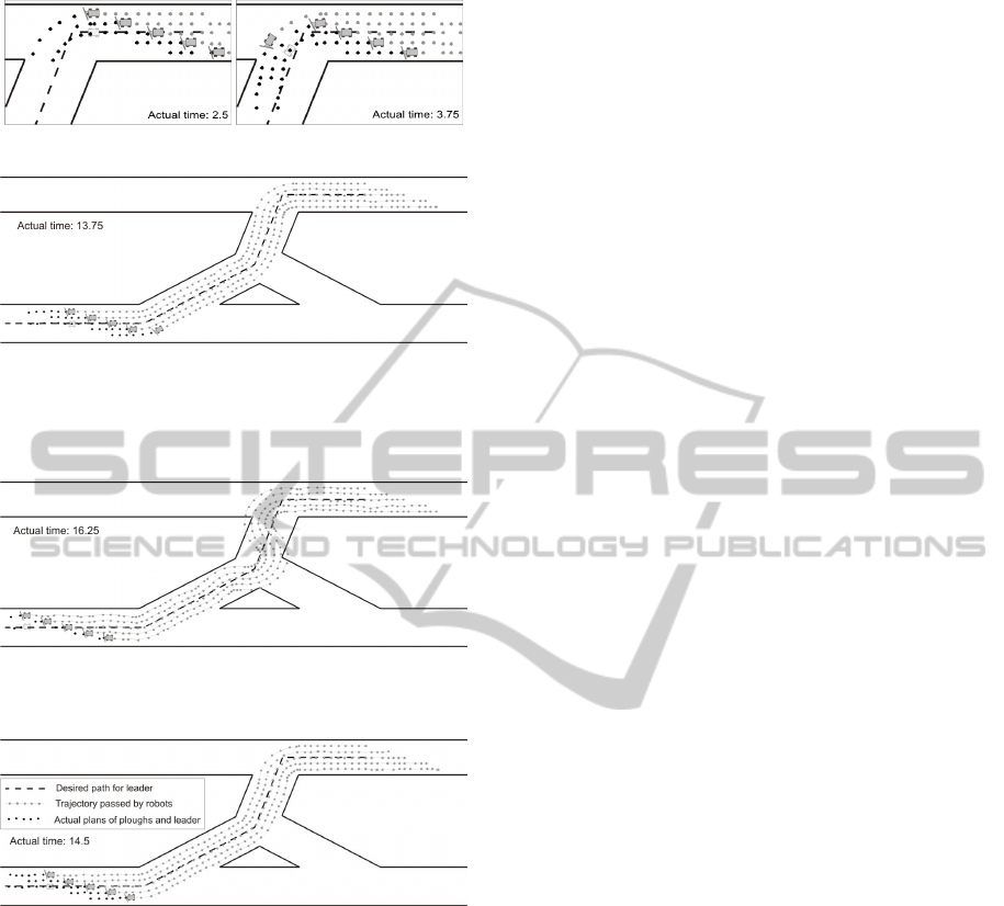
(a) The ﬁrst response to the path

break.

(b) The ﬁrst plough turns deviated

from the optimal way.

jectories.

Figure 3: Formation driving algorithm with parameters N =

6 and n = 5.

Figure 4: Formation driving algorithm with parameters N =

2 and n = 1.

Figure 5: Formation driving algorithm with parameters N =

6 and n = 2.

ploughs as well as for the virtual leader and the grey

points denote states visited during the previous move-

ment. The dashed line represents the desired path that

has to be followed by the virtual leader that is drawn

by a contour in front of the formation.

The ﬁrst snapshot in Fig. 2(a) was captured at time

when the ﬁrst response to the approaching change of

heading is enabled. Nevertheless, it is too late to come

through the curve optimally and so the deviation from

the second path segment produces an uncleaned part

of the runway (see Fig. 2(b)).

The second problem, the interval n being too long,

is clariﬁed in Fig. 3 where the algorithm with n = 5

and N = 6 was utilized. Again the ﬁrst snapshot in

Fig. 3(a) was captured at time of the ﬁrst possible re-

sponse to the path break. As one can see, the for-

mation is already too close to the line break due to

the long period where the robots just blindly executed

preplanned control inputs. Therefore, the ploughs

again overshoot the desired path (see Fig. 3(b)). Re-

sults of the simulation with the setting of parameters

n = 2 and N = 6 are presented in Fig. 5 for compari-

son.

4 CONCLUSIONS

In this paper, we have described an approach of for-

mation driving. The method is based on a model pre-

dictive control extended by an additional time horizon

for navigation to a target region. The robustness of

the algorithm and the inﬂuence of its parameters on

the system performance were veriﬁed by simulations.

ACKNOWLEDGEMENTS

This work is supported by GA

CR under the grant no.

P103-12/P756 and by M

SMT under the grant COLOS

no. LH11053.

REFERENCES

Barfoot, T. D. and Clark, C. M. (2004). Motion planning for

formations of mobile robots. Robotics and Autonom.

Syst., 46:65–78.

Chen, J., Sun, D., Yang, J., and Chen, H. (2010).

Leader-follower formation control of multiple non-

holonomic mobile robots incorporating a receding-

horizon scheme. Int. J. Rob. Research, 29:727–747.

Dunbar, W. and Murray, R. (2006). Distributed receding

horizon control for multi-vehicle formation stabiliza-

tion. Automatica, 42(4):549–558.

Liu, Y. and Jia, Y. (2012). An iterative learning approach to

formation control of multi-agent systems. Systems &

Control Letters, 61(1):148 – 154.

Mayne, D. Q., Rawlings, J. B., Rao, C. V., and Scokaert, P.

O. M. (2000). Constrained model predictive control:

Stability and optimality. Automatica, 36(6):789–814.

Saska, M., Hess, M., and Schilling, K. (2008). Efﬁcient air-

port snow shoveling by applying autonomous multi-

vehicle formations. In Proc. of IEEE ICRA.

Saska, M., Vonasek, V., and Preucil, L. (2011). Formation

coordination with path planning in space of multino-

mials. In Artiﬁcial Intelligence and Soft Computing.

Zhang, F. (2010). Geometric cooperative control of par-

ticle formations. IEEE Trans. on Autom. Control,

55(3):800 –803.

ICINCO2012-9thInternationalConferenceonInformaticsinControl,AutomationandRobotics

406