Control and Model Parameters Identification of Inertia Wheel Pendulum
Paweł Drapikowski, Jarosław Go
´
sli
´
nski and Adam Owczarkowski
Institute of Control and Information Engineering, Pozna
´
n University of Technology, Piotrowo 3a, 60-965 Pozna
´
n, Poland
Keywords:
Inertia Wheel Pendulum, Kalman Filter, Extended Kalman Filter, Linear-Quadratic Regulator.
Abstract:
This paper presents control method of an inverted pendulum with an inertial drive (IWP Inertia Wheel Pen-
dulum). This is a non-linear, underactuated mechanical system and therefore it has more degrees of freedom
than control variables. In application, electric motor has been placed on the pendulum top and it is a source of
torque, which accelerates the flywheel. Position of the pendulum depends on the acceleration of the flywheel.
This paper shows algorithm for the real object to keep the inertia wheel pendulum in the vertical position
at equilibrium point. In order to achive this aim, authors decided to concentrate on modern and advanced
techniques of control and estimation such as LQR regulator, sensor fusion, extended Kalman Filter and model
parameters identification.
1 INTRODUCTION
Control of an inverted pendulum is a well known
problem (Bradshaw and Shao, 1996). There are many
control methods and different types of inverted pen-
dulum. One of the most interesting pendulum con-
struction is the inertia wheel pendulum (Spong and
P. Corke, 1999). It has got motor with attached fly-
wheel, located on the top. Many times, this kind of
pendulums are only subject of simulation. In this pa-
per, control problem as well as hardware implemen-
tation is presented. For the future research purpose,
authors developed IWP with addidional wheels on the
bottom (mobile robot), as shown in Fig. 1.
Figure 1: IWP - real photo.
In this independend IWP platform, absolute posi-
tion and velocity sensor were needed as well as proper
control algorithm. For needs of this application, sen-
sor fusion algorithm was used (given in section 2) and
also Extended Kalman Filter (stated in section 3). It
can be seen that with filter algorithm of Kalman func-
tion, control will be based on Linear-Quadratic prob-
lem, which is true and described in section 4. During
further steps, authors decided to involve model pa-
rameters identificator in order to keep control gain up
to date and to track for object parametrs change. Iden-
tifcation methods are stated in section 5. The overall
control scheme of the IWP is shown in Fig.2.
Figure 2: Overall control scheme.
2 SENSORS AND FUSION
ALGORITHM
Measurement unit consists of absolute sensors i.e. gy-
574
Drapikowski P., Go
´
sli
´
nski J. and Owczarkowski A..
Control and Model Parameters Identification of Inertia Wheel Pendulum.
DOI: 10.5220/0003990405740579
In Proceedings of the 9th International Conference on Informatics in Control, Automation and Robotics (ICINCO-2012), pages 574-579
ISBN: 978-989-8565-21-1
Copyright
c
 2012 SCITEPRESS (Science and Technology Publications, Lda.)

roscope and accelerometer. Problem of noisy signals
has led to choose uncommon version of the Kalman
filter for sensor fusion. It takes simultaneously two
signals: from the gyroscope and from the accelerom-
eter. This sensors fusion has two major advantages.
Firstly, it gives better angle estimation when inte-
grating gyroscope result than taking raw data directly
from accelerometer. Secondly, it provides estimation
without bias, when taking into account accelerometer
measurements (as a reset function for the qyroscope
integrator bias).
For better understanding fusion algorithm, short
description about sensors location must be given. The
main gyrocope axis lies in line with Y IWP’s axis and
active accelerometer axis is parallel to X pendulum’s
axis. This allows to concatenate measurements re-
sults from gyroscope and accelerometer sensors. Ac-
celerometer works here as an inclinometer and gy-
roscope as an angle velocity meter. In Kalman Fil-
ter configured for a sensor fusion given by following
equations:
Prediction
ˆx
−
k
= A · ˆx
k−1
+ B · u
k−1
P
−
k
= A · P
k−1
· A
T
+ Q
(1)
Correction
K
k
= P
−
k
·C
T
· (C · P
−
k
·C
T
+ R)
−1
ˆx
k
= ˆx
−
k
+ K
k
· (z
k
−C · ˆx
−
k
)
P
k
= (I − K
k
·C) · P
−
k
(2)
matrices A, B, C shape mathematical model of the
measurement system (fusion). For matrices:
A =


1 0 −dt
0 0 −1
0 0 1


, B =


dt
1
0


(3)
C =

1 0 0

(4)
* where dt is equal to integration interval
and input signal u
k
(equal to gyroscope mea-
surement) as well as input z
k
(equal to accelerometer
declination) it is possible to perform sensor fusion.
This algorithm has two inputs: angle velocity and
declination. In Eqns. (1) and (2), ˆx
−
k
and ˆx
k
stand
for estimation vector (a priori and a posteriori,
respectively). During the process of fusion, three
values are estimated:
ˆx = [
ˆ
α,
ˆ
˙
α,
ˆ
ζ]
T
(5)
ˆ
α stands for an IWP angle,
ˆ
˙
α is equal to angular ve-
locity and finally
ˆ
ζ is an angular velocity bias (offset),
which must be known in order to improve angle ve-
locity estimation.
3 EXTENDED KALMAN FILTER
During the work also has taken advantage of extended
Kalman filter. It uses two groups of input signals:
measurements (with fusion results) and excitation of
the object (which is equal to current). By using
Kalman Filter it is possible to predict next state of
the IWP. For this purpose desired values (angle, an-
gular velocity of the pendulum and the angular veloc-
ity of the flywheel) and input signal are needed. This
Kalman Filter is based on IWP’s mathematical model.
Model can be given by IWP matrices: (6), (7),(8) and
(9).
A
k
=



1 T
p
0
m
c
gl
p
sin(α)
I
r
+I
k
T
p
1 −
b
α
I
r
+I
k
T
p
−
b
φ
I
r
+I
k
T
p
0 0 1 −
b
φ
I
k
T
p



(6)
B
k
=


0
k
I
r
+I
k
T
p
k
I
k
T
p


(7)
C
k
=


1 0 0
0 1 0
0 0 1


(8)
D
k
=


0
0
0


(9)
As it has already been stated excitation signal for
the IWP is current, which flows through the DC mo-
tor. To make this current controllable, it was obliga-
tory to use current regulator. It has been completed
with current regulator directly in the plant. Thus,
model above is current driven.
IWP’s model is nonlinear (matrix 6). There-
fore, in order to estimate state vector, authors had
to use extended Kalman filter. This estimator can be
stated as a two-phase algorithm. In first phase IWP’s
model is stimulated by current value, (calculated from
the IWP’s position regulator), then covariance matrix
(P
−
k
) projection is made. First phase is given by group
of equations (10):
ˆx
−
k
= f
k
( ˆx
k−1
, u
k−1
)
F
k
=
∂ f (ˆx
k−1
,u
k−1
)
∂ ˆx|
ˆx= ˆx
k−1
=
∂[A
k
· ˆx
k−1
+B
k
·u
k−1
]
∂ ˆx|
ˆx= ˆx
k−1
P
−
k
= F
k
· P
k−1
· F
T
k
+ Q
k
(10)
In the second phase, whole state ( ˆx
−
k
), estimated in
the first phase is corrected. During this stage angular
velocity from IWP’s wheel and estimates from sensor
fusion are taken into account as a vector z
k
. Correc-
tion phase is as follows:
ControlandModelParametersIdentificationofInertiaWheelPendulum
575

H
k
=
∂h( ˆx
k−1
)
∂ ˆx|
ˆx= ˆx
k−1
=
∂[C
k
· ˆx
k−1
]
∂ ˆx|
ˆx= ˆx
k−1
K
k
= P
−
k
· H
T
k
· (H
k
· P
−
k
· H
T
k
+ R
k
)
−1
ˆx
k
= ˆx
−
k
+ K
k
· (z
k
−C
k
· ˆx
−
k
)
P
k
= (I − K
k
· H
k
) · P
−
k
(11)
In correction phase Kalman gain (K
k
) is calculated
as well as an ultimate state vector ( ˆx
k
). Finally, covari-
ance matrix is updated.
4 OBJECT PARAMETERS
IDENTIFICATION
Identification process was introduced in order to track
change of the model parameters. Among many sys-
tem identification methods, there are a few which can
be used in this work. Before selecting indetification
method it is necessary to choose proper structure for
the model. One of the best structure (due to the sim-
plicity of its implementation) is ARX (Autoregressive
Exogenous model). Frame for this structure is given
by following equation:
y
k
=
B(q
−1
)
A(q
−1
)
u
k−d
+
1
A(q
−1
)
e
k
(12)
* where d > 0 and:
A(q
−1
) = 1 +a
1
q
−1
+ ... + a
n
q
−n
B(q
−1
) = b
0
+ b
1
q
−1
+ ... + b
m
q
−m
For the model description, ARX structure (12) can be
taken into consideration but only under the assump-
tion that IWP’s model is linearized. As has already
been stated, IWP’s model is nonlinear (sin function
in (6)). This must be eliminated from model. Model
also has to take shape of transitional equations which
can be derived from IWP’s matrices (6), (7),(8) and
(9):
α
k
= α
k−1
+
˙
α
k−1
T
p
(13)
˙
α
k
=
m
c
gl
p
I
r
+I
k
sin(α
k−1
) + (1 −
b
α
T
p
I
r
+I
k
)
˙
α
k−1
+
+(−
b
φ
T
p
I
r
+I
k
)φ
k−1
+
kT
p
I
k
+I
r
i
(14)
φ
k
= (1 −
b
φ
T
p
I
k
)φ
k−1
+
kT
p
I
k
i
k−1
(15)
As it can be seen, Eqn. (13) is only additional and
there are no parametres to be identified. Second equa-
tion (14) which forms the model cannot be written in
a ARX structure directly, without modifications. To
do so, it is necessary to eliminate term with sin func-
tion (which depends on α parameter). In order to this,
whole term with sin function has to be included to a
known disturbance e
k
:
e
k
=
m
c
gl
p
I
r
+I
k
sin(α
k−1
) + ξ
(16)
* where ξ is additional noise
Furthermore, equation (14) has two inputs i.e.
variable φ and i. For needs of the ARX structure
it is desirable to have only one input variable and
one output variable. This can be achieved by proper
substitution of equation (15) into equation (14). From
(15) following equation can be derived:
I
k
I
k
+I
r
φ
k
−
I
k
I
k
+I
r
φ
k−1
= −
b
φ
T
p
I
k
+I
r
φ
k−1
+
kT
p
I
k
+I
r
i
(17)
which can be substituted to (14). After substituting,
new system of equations will be obtained:
φ
k
= (1 −
b
φ
T
p
I
k
)φ
k−1
+
kT
p
I
k
i
k−1
(18)
˙
α
k
= (1 −
b
α
T
p
I
r
+I
k
)
˙
α
k−1
+
I
k
I
k
+I
r
φ
k
−
I
k
I
k
+I
r
φ
k−1
+ e
k
(19)
From this point, system consists of two equations
((18) and (19)). These equations are suitable for ARX
structure. Only in equation (19) it might be seem, that
the delay parameter d is not greater then zero (ARX
structure, eqn. (12)), which does not allow the pro-
cess to be correct. Nevertheless, in this particular case
φ
k
can be taken directly from the eqn. (18) which is
normally calculated before
˙
α
k
.
In order to perform identification process least
squares method has been selected. Identification pro-
cess must be executed as an online algorithm. This
can be accomplished by use of the recursive least
squares method (RLS) which is given by equations
(20)-(23)
ˆ
θ
k
=
ˆ
θ
k−1
+
P
k−1
ϕ
k
λ
k
+ ϕ
T
k
P
k−1
ϕ
k
ε
k
(20)
P
k
= (P
k−1
−
P
k−1
ϕ
t
ϕ
T
k
P
k−1
λ
k
+ ϕ
T
k
P
k−1
ϕ
k
)
1
λ
k
(21)
ε
k
= y
k
− ϕ
T
k
ˆ
θ
k−1
(22)
λ
k
= λ
0
λ
k−1
+ (1 − λ
0
) (23)
For each of the final model equations (i.e. (18) and
(19)) procedure of the RLS must be carried out. After
each iteration of the RLS, results are available in
ˆ
θ
k
vector. For the equation (18) it can be written that:
ˆ
θ
k
=
h
(1 −
b
φ
T
p
I
k
)
kT
p
I
k
i
T
(24)
and for equation (19) it is true that:
ˆ
θ
k
=
h
(1 −
b
α
T
p
I
r
+I
k
)
I
k
I
k
+I
r
I
k
I
k
+I
r
i
T
(25)
ICINCO2012-9thInternationalConferenceonInformaticsinControl,AutomationandRobotics
576

At this point very important is to set proper values for
the forgetting factor λ
0
and λ
0
. For maximum value
of 1, whole algorithm will be not sensitive for pa-
rameters change. On the other hand, small values for
λ’s can make RLS method internally unstable, which
could be observed as a oscillation in parameters.
5 LQR REGULATOR
The control system uses a linear quadratic regulator
LQR. It includes changing in time model which is lin-
earized in every point of trajectory. This solution is
suitable for stabilizing non-linear systems and it has
adaptive nature.
The LQR regulator can be applied to non-linear
system which is linerized along the trajectory. Then
the system matrices change in time.
The control aim is to make every state variable as
a desired value which is zero. The feedback uses the
whole state vector. Regulation system is in Fig. 3.
Figure 3: The LQR regulation system.
The control law is based on the optimal criterion
given by equation:
J =
n
∑
i=0
"
x
T
i
Q
LQR
x
i
+ R
LQR
u
2
i
#
, (26)
where Q
LQR
= Q
T
LQR
, J is quadratic cost function, x
i
is a state vector, u
i
is a control vector, n is a number
of iteration in regulator calculation process, Q
LQR
is a
state weight matrix and R
LQR
is weight of control sig-
nal. The aim is to minimize that quadratic criterion.
R
LQR
and Q
LQR
have constant values ((Wang et al.,
2010), (Zhang and Wang, 2010)):
R
LQR
= 100, (27)
Q
LQR
=


1 0 0
0 1 0
0 0 1


. (28)
This paper shows discrete time form of LQR equa-
tions with finite horizon which made it easer to imple-
ment it in the real application. In (Zabczyk, 1991) it
is shown how difficult solving continuous time LQR
equations is. For discrete problem it is needed to have
discrete state space model:
x
k+1
= A
d
x
k
+ B
d
u
k
, (29)
y
k
= C
d
x
k
+ D
d
u
k
, (30)
where A
d
, B
d
, C
d
and D
d
are discrete model matrices.
The author of (Sauer, 2011) describes how to obtain
them having linear model matrices. Here was used
approximate iterative method.
The control law is given by:
u
k+1
= −K
k
x
k
, (31)
where K
k
is a gain vector which equals to:
K
k
= (R
LQR
+ B
T
d
P
k
B
d
)
−1
B
T
P
k
A
d
. (32)
The P
k
is only unknown value which is the solution of
an iterative backward discrete time Riccati equation
((Yishao, 1996)):
P
k−1
= Q
LQR
+A
T
d
(P
k
−P
k
B
d
(R+B
T
d
P
k
B
d
)
−1
B
T
d
P
k
)A
d
,
(33)
with initial value P
n
= Q
LQR
. Sometimes it is
called ILQR (Iterative Linear Quadratic Regulator)
like in (In-Won et al., 2010) and (Li and Todorov,
2004).
6 RESULTS
In order to check every mentioned algorithms a proto-
type of an IWP was built. Using the computer simu-
lation acceptable mechanical parameters were found.
As a measurement unit, inertial sensor ADIS16355
from Analog Devices Company was used. It has high
precision tri-axis gyroscope and accelerometer. The
second important thing was the implemented – high
torque, DC current motor. It was direct drive for the
flywheel. Direct drive generates much less vibrations
than any mechanical transmissions. The last essential
thing was well-balanced flywheel. Every calculations
were made by using a personal computer.
Sensor fusion was the first thing, that authors had
to prepare and then check. In Fig. 4 comparison of
results of the Kalman Filter fusion is shown.
As it can be seen, accelerometer generates signal
with additional noise which is (i.a.) dynamic accel-
eration. In normal operation, it is impossible to esti-
mate declination from the pivot point by using only
accelerometer. By using fusion with gyroscope good
estimation can be obtained. In this example, authors
used proper settings for the fusion algorithm which
is: small variance (Q=0.0001) for gyroscope signal
and large variance (R=0.1) for accelerometer signal.
Right after fusion, algorithm of Extended Kalman
Filter performs his action. One of the estimates is
shown in Fig. 5. It is easy to see that Extended
Kalman Filter gives the opportunity to make estimates
robust for the noise, even from optical encoder. The
ControlandModelParametersIdentificationofInertiaWheelPendulum
577

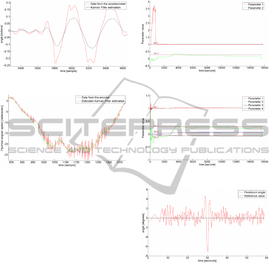
Figure 4: Measurement from accelerometer (red line) and
fusion result (black line) - comparison.
Figure 5: Measurement from the encoder (red line) and its
Extended Kalman Filter estimation (green line) - compari-
son.
estimations from identification module are as impor-
tant as those from Kalman filter. In Fig. 6 and 7 iden-
tification results are shown. First figure shows results
for the vector (24) and the second one, shows results
for (25) (with addional error estimation - red line).
As it can be seen, identification gives good results
(blue line is the reference, theoretical value for each
of parameter), but for the RLS algorithm, where there
are more then two parameters for the identifiacation it
is necessary to wait about 16 seconds (4000 samples
with rate of 250 sample/sec).
Last thing was the regulator. The LQR regulation
worked properly, because it was possible to stabilize
the pendulum in vertical position. Every three state
variables were close to zero value during the experi-
ments. Trajectory of the first state variable is shown
in Fig. 8.
Finally the pendulum was able to stand in the ver-
tical position in infinite time horizon. The maximum
amplitude of the first state variable was 2.5 degree.
The angle of 9 degrees was the biggest possible exter-
nal disturbance that has not led to the collapse.
Figure 6: Identification results (1). Two parameters from
Eq. (24) with their reference values.
Figure 7: Identification results (2). Four parameters from
Eq. (25) with their reference values.
Figure 8: Experimental trajectory of the first state variable
(angle from vertical position).
7 CONCLUSIONS
The experiment confirmed the theoretical considera-
tions. It was possible to achieve satisfactory results
through a combination of Kalman filter, identifica-
tion and LQR regulation. Though, whole application
working fine, results of algorithm of the parameters
identification are not as good as they were expected
to be. In this case, changes track of the parameters
can lead to dangerous situations, such as sudden an-
gle growth or decrease (LQR depends on identifica-
ICINCO2012-9thInternationalConferenceonInformaticsinControl,AutomationandRobotics
578

tion process). Therefore it is recommended to take
some precautions for example: software conditions
that make the identificator supervised. However, the
above solution shows that the creation of innovative
electric vehicles with inertia stabilization is possible.
In the future personal computer will be replaced by
DSP microcontroller or FPGA device. This may help
in creating a fully independent stabilization unit.
REFERENCES
Bradshaw, A. and Shao, J. (1996). Swing-up control of in-
verted pendulum systems. volume 14, pages 397–405.
Robotica.
In-Won, P., L. Bum-Joo, K. Y.-H., Ji-Hyeong, H., and Jong-
Hwan, K. (2010). Multi-objective quantum-inspired
evolutionary algorithm-based. IEEE World Congress
on Computational Intelligence, pages 18–23.
Li, W. and Todorov, E. (2004). Iterative linear quadratic reg-
ulator design for nonlinear biological movement sys-
tems. In in Proc. of Int. Conf. on Informatics in Con-
trol, pages 1–8, Setubal Portugal.
Sauer, P. (2011). Sterowanie procesami ciagymi i dyskret-
nymi – liniowe dyskretne rownania stanu.
Spong, M. W. and P. Corke, R. L. (1999). Nonlinear con-
trol of the inertia wheel pendulum. In research un-
der grants CMS-9712170 and ECS-9812591, Urbana,
Kenmore, France.
Wang, H., Dong, H., He, L., Shi, Y., and Zhang, Y. (2010).
Design and simulation of lqr controller with the linear
inverted pendulum. In International Conference on
Electrical and Control Engineering, China.
Yishao, Z. (1996). Convergence of the discrete-time riccati
equation to its maximal solution. In Department of
Mathematics Stockholm University, Sweden.
Zabczyk, J. (1991). Zarys matematycznej teorii sterowania.
Wydawnictwo Naukowe PWN.
Zhang, B. and Wang, J. G. (2010). The analysis and simu-
lation of first-order inverted pendulum control system
based on lqr. In Third International Symposium on
Information Processing, China.
ControlandModelParametersIdentificationofInertiaWheelPendulum
579