Semi-static Object Detection using Polygonal Maps for Safe Navigation

of Industrial Robots

Dario Lodi Rizzini, Gionata Boccalini and Stefano Caselli

Dipartimento di Ingegneria dell’Informazione, University of Parma, viale G.P. Usberti 181A, 43124 Parma, Italy

Keywords:

Mapping, Range Sensing.

Abstract:

The collision and safety control of industrial UGVs equipped with laser range ﬁnders is often based on con-

servative area-oriented policies that lack in ﬂexibility and does not deal well with non ephemeral environment

changes due to semi-static objects (e.g. passive misplaced objects). In this paper, we propose a method to de-

tect and represent semi-static objects using polygonal local maps in order to improve robot navigation. Each

local map consists of polylines representing the boundary of an object detected inside a safety area. Polylines

are extracted from laser scans and associated with the polylines of a reference map using a similarity measure

criterion. Finally, the map is updated by merging the new polylines. The proposed polygonal representation

allows the recognition of new semi-static obstacles in the environment and supports more ﬂexible policies for

safe navigation. An EKF localizer using artiﬁcial landmarks and a ﬁxed path navigation system have been im-

plemented to replicate the navigation system of industrial UGVs. The precision of environment reconstruction

has been assessed with experiments in simulated and real environments.

1 INTRODUCTION

Unmanned Ground Vehicles (UGVs) are more and

more used to manage logistics, individually or in co-

ordinated teams, in industrial plants and warehouses.

Being completely autonomous, these vehicles are

usually equipped with laser range ﬁnders to perceive

obstacles and to localize and navigate in the environ-

ment. Laser range ﬁnders for localization are usu-

ally mounted on the LGV top to avoid occlusions and

to perceive artiﬁcial landmarks with high remission

value that have been previously placed in the envi-

ronment. An Extented Kalman Filter (EKF) local-

izer tracks and estimates the pose of the robot using

the observed landmarks and an a priori map of the

landmarks. Safety lasers (e.g. Sick S300) are usu-

ally placed slightly above ﬂoor level for the detec-

tion of any object lying in the proximity of the robot.

One common safety policy consists of partitioning the

space in front of the laser idle, warning and protective

areas. The warning and the protective areas are sup-

posed to be free in normal working conditions so an

appropriate size for the areas must be deﬁned for each

segment of the LGV trajectory. When an object is per-

ceived in the warning area (shown in yellow in bottom

of Figure 1), the UGV slows down according to the

warning. When the protective area (in red in Figure 1)

is not free, the vehicle stops. For any plant operating

with LGVs, the dimensions of warning and protective

areas vary in the different regions of the working en-

vironment. This strict and conservative policy grants

the safety of people and things, but it is inefﬁcient and

inﬂexible. Sizing the safety areas is a time-consuming

and tedious operation that must be repeated whenever

the environment layout changes. Furthermore, while

it is mandatory that the robot stops when a collision

with a person or an obstacle may occur, the efﬁciency

of the system is often affected by objects thought-

lessly left in the assumed free space. Although the

area classiﬁcation scheme has been conceived to en-

sure safety margin in presence of human operators,

the majority of reduction in UGV navigation speed is

actually due to passive misplaced objects. These ob-

jects may be modeled as semi-static objects that do

not belong to the persistent structure of the environ-

ment. Semi-static objects change their location with

low frequency (e.g. after several hours) and while the

robot is not observing them.

In this paper, we propose a method to detect and

represent semi-static objects using polygonal local

maps in order to improve robot navigation. In the pro-

posed solution, the representation of semi-static ob-

jects is assigned to a collection of local maps where

each local map covers a speciﬁc path segment. Local

maps are more manageable than a single global map

and can be more easily integrated with the existent

191

Lodi Rizzini D., Boccalini G. and Caselli S..

Semi-static Object Detection using Polygonal Maps for Safe Navigation of Industrial Robots.

DOI: 10.5220/0003989601910198

In Proceedings of the 9th International Conference on Informatics in Control, Automation and Robotics (ICINCO-2012), pages 191-198

ISBN: 978-989-8565-22-8

 2012 SCITEPRESS (Science and Technology Publications, Lda.)

navigation system. Such maps consist of polygonal

lines or, shortly, polylines that represent the bound-

ary of the obstacles found inside the warning and

protective areas. Polygonal representation is mem-

ory and bandwidth inexpensive, compact and seman-

tically rich. A similarity measure is used to asso-

ciate the observed polylines with a preexisting map

for robust detection of semi-static objects. When a

semi-static object is found inside a safety area, the

corresponding local map is updated and the dimen-

sion of the safety areas of the laser range sensor may

be adapted to the reduced free space. Thus, the next

LGV visiting the same region is not forced to slow

down or to stop since the updated area does not con-

tain semi-static object. More advanced and efﬁcient

policies may be implemented by giving up the con-

servative safety area. The proposed approach has

been assessed in simulation and in a real experimen-

tal setup. For this purpose, an EKF localizer based on

landmark and a navigation system have been imple-

mented.

2 RELATED WORK

Research on robot localization and map building early

met the problem of representing dynamics in the en-

vironment. The ﬁrst and most common approach is

the removal of moving objects when detected. Fox

et al. (Fox et al., 1999) proposed a sensor model

for range ﬁnders that can deal with dynamic objects

by modeling them as noise. The work of Wolf et

al. (Wolf and Sukhatme, 2005) is one of the ﬁrst si-

multaneous localization and mapping (SLAM) meth-

ods that explicitly distinguishes between dynamic en-

tities and static environments using two different oc-

cupancy grid maps. Stachniss et al. (Stachniss and

Burgard, 2005) focus on the semi-static objects, i.e.

objects that infrequently change their location while

the robot is not observing them. Semi-static objects

like doors, parking locations, etc., often deﬁne the

discrete state of the environment providing also long-

term semantic information. Recent localization meth-

ods represent static, semi-static and dynamic objects

in the map (Meyer-Delius et al., 2010). The majority

of these techniques are based on an occupancy grid

map, which is suitable to integrate range measure-

ments into a robust representation of the environment,

but it does not carry shape or semantic information

(an object corresponds to a group of cells) and is not

apt to be shared among distributed robots.

Several other works identiﬁes either generic (Katz

et al., 2008) or speciﬁc moving entities like peo-

ple (Spinello et al., 2009) from consecutive range

measurements. Tipaldi and Ramos (Tipaldi and

Ramos, 2009) proposed a method performing simul-

taneously scan matching and moving cluster detection

using Conditional Random Fields (CRF). These ap-

proaches are oriented only to the detection and short-

term tracking of people and objects and represent

their targets as clusters of points.

Strict-sense polygonal representations have not

been extensively used for mapping, since a polyline is

a composite element and cannot be represented with

a ﬁxed number of variables as would be convenient

for state estimation algorithms like Bayesian ﬁlters.

On the other hand, EKF localization and mapping al-

gorithms often utilize line segment feature maps ac-

cording to models like SP-map models (Arras, 2003).

Latecky et al. (Latecki et al., 2004) illustrated a tech-

niques for integrating the polylines extracted by range

measurements by exploiting shape similarity measure

and scan order.

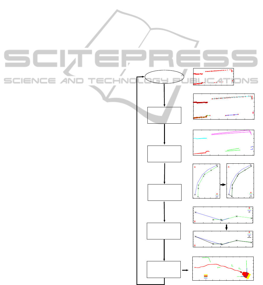
Laser scan

Polyline

extraction

-0.5

0.5

1.5

2.5

0 1 2 3 4 5 6 7

-0.5

0.5

1.5

2.5

0 1 2 3 4 5 6 7

Polyline

association

Polyline

merge

Polyline

join

-0.3

-0.2

-0.1

0.1

0.2

0.3

0.4

0.5

0.6

10 10.5 11 11.5 12 12.5 13

Point of view

New polyline points

New polyline

-3

-2.5

-2

-1.5

-1

-0.5

0 0.5 1 1.5 2

Point of view

New polyline points

New polyline

-3

-2.5

-2

-1.5

-1

-0.5

0 0.5 1 1.5 2

Point of view

New polyline points

-0.3

-0.2

-0.1

0.1

0.2

0.3

0.4

0.5

0.6

10 10.5 11 11.5 12 12.5 13

Point of view

New polyline points

Map

update

-2

-1.5

-1

-0.5

0.5

1.5

1 2 3 4 5 6 7 8 9 10

Warning area

Protective area

Map

Current scan

Robot poses

-0.5

0.5

1.5

2.5

0 1 2 3 4 5 6 7

Figure 1: Diagram illustrating the algorithm for building

polygonal maps from laser scans.

ICINCO2012-9thInternationalConferenceonInformaticsinControl,AutomationandRobotics

192

3 POLYGONAL MAP

REPRESENTATION

This work aims to detect and track the non ephemeral

changes occurring inside the region of environment

covered by the robot range sensors. The robot moves

along a collection of path segments deﬁned a priori.

On each path segment a speciﬁc safety area (consist-

ing of warning and protective areas) is deﬁned to de-

tect potential obstacles without including the static

part of environment. When a stationary entity is de-

tected inside a safety area, the system should record

such semi-static object in a map of the environment.

Instead of managing a single global map, the natu-

ral segmentation of the robot path can be exploited to

cover the working environment with more manage-

able local maps of limited dimensions. The reference

frames of these local maps are anchored to the refer-

ence frame on the path segments.

A local map consists of polygonal lines or poly-

lines that are represented by the list of their vertices.

Polylines are compact geometric features that repre-

sent the countour of obstacles and that can be easily

extracted by laser range scans. Polygonal maps meet

several of the system requirements. First, polylines

require limited storage and bandwidth for their trans-

mission among the LGVs working together in the en-

vironment. Second, the result of polylines extraction

from laser scan is already a segmented set since each

polyline represents an object or a portion of an ob-

ject, though the extraction algorithm must handle er-

rors due to occlusions and sensor noise. Finally, poly-

lines encode shape information that would be implicit

in occupancy grid representations and that can be ex-

ploited for robust data association.

The steps of the algorithm for extracting and inte-

grating the polylines from the laser scan into a consis-

tent map are illustrated in Figure 1. The algorithm ex-

tracts polylines from current laser scan (polyline ex-

traction) and associates them with the polylines con-

tained in the existing map using the similarity mea-

sure (polyline association). Then, the scan polylines

are merged with the associated elements of the map

(polyline merge). Finally, the close polygonal lines

are joined to remove inconsistent and redundant items

(polyline join). In the following, the details of the pro-

posed algorithm are discussed.

3.1 Polyline Extraction

Polylines are extracted from each raw laser range scan

by removing outliers, by splitting the scan into inter-

vals and ﬁnally by choosing the vertices of the poly-

lines. Scans are commonly represented as sorted vec-

tors of ranges or, equivalently, of points (symbols r

and p

will refer to range or Cartesian point hence

after). The implicit angular order of ranges is used

by the standard extraction techniques (Xavier et al.,

2005) as those applied in this work.

First processing step is the statistical out-

lier removal. For each window of ranges

i−k

, . . . , r

i+k

centered on i −th range the mean

value µ

and standard deviation σ

are computed. The

two statistics are used to detect isolated measure-

ments. If the difference between range r

and win-

dow mean value µ

is greater than a threshold α σ

(α is a parameters set by the user), then measurement

i is removed from the scan. The scan is then split

into intervals in correspondence to a strong disconti-

nuity between consecutive ranges. The discontinuity

is detected according to the standard adaptive thresh-

old criterion. The line connecting two consecutive

discontinuous points represents the border of the oc-

cluded region.

Each scan interval corresponds to a polyline repre-

senting an object or a part of an object. All the points

of an interval may serve as vertices of the polyline.

However, when points are approximatively aligned,

the polyline is better represented by a less redundant

list of points. Such result can be easily achieved us-

ing Douglas-Peuker algorithm for curve simpliﬁca-

tion (Douglas and Peuker, 1973). A similar result

could be obtained using the discrete curve evolution

(DCE) proposed in (Latecki et al., 2004).

3.2 Metric for Polylines

The association of polylines belonging to different

sets is a crucial operation for the construction of lo-

cal map and for the detection of the objects that have

been already observed or not yet observed. Associ-

ation is performed on two sets of polylines, i.e. the

polylines extracted from the laser scan and the poly-

lines belonging to the existing local map. Polyline

association requires a metric to measure the likeness

of a single pair of polylines and a procedure to esti-

mate the most consistent joint set of associated pairs.

The latter aspect is discussed in the next section.

In this work, two different metrics are used. The

ﬁrst one aims at measuring the shape similarity be-

tween two polylines. The second estimates a bound

on the Euclidean distance between the points of two

polylines to validate the similarity. Since the robot

pose can be accurately estimated using a localizer, the

pose of polylines in the map is accurate enough to use

proximity as a validation of data association.

Two simple curves in the plane are perceived as

similar if their tangent vector “turns” in the same way.

Semi-staticObjectDetectionusingPolygonalMapsforSafeNavigationofIndustrialRobots

193

0.4

0.5

0.6

0.7

0.8

0.9

1.1

1.2

0 0.2 0.4 0.6 0.8 1 1.2 1.4 1.6

0.4

0.5

0.6

0.7

0.8

0.9

1.1

1.2

0 0.2 0.4 0.6 0.8 1 1.2 1.4 1.6

0.5

1.5

2.5

3.5

0 0.2 0.4 0.6 0.8 1

Hystogram Polyline 0

0.5

1.5

2.5

3.5

0 0.2 0.4 0.6 0.8 1

Hystogram Polyline 1

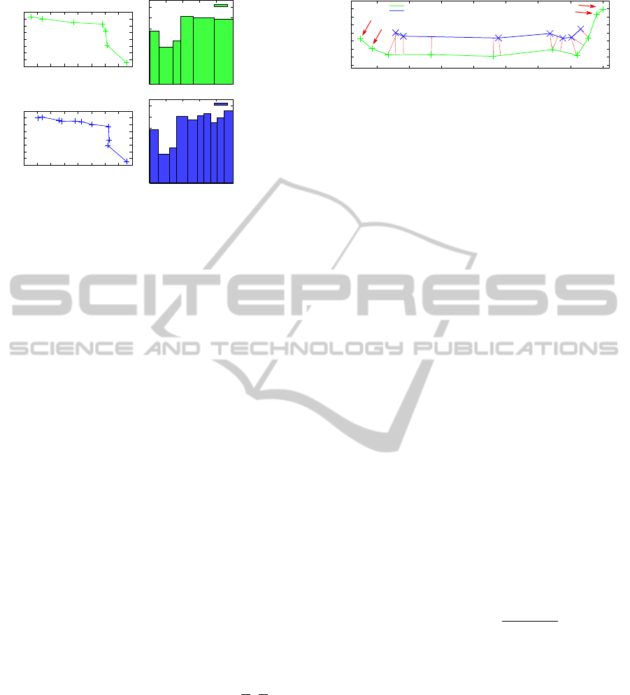
Figure 2: Polyline shape similarity of polyline 0 (top-left)

and polyline 1 (bottom-left) is measured comparing their re-

spective tangent space histograms (top- and bottom-right).

The concept of similarity has been originally formal-

ized in (Latecki and Lakaemper, 1999) for closed

polygons and then extended to polylines (Latecki

et al., 2004). The idea is to compare the normal-

ized tangent histograms of two polylines P

and P

The polygonal curves P

s and P

s are parameterized

w.r.t. their normalized arclength s ∈ [0, 1]. The tan-

gent function T

(s) : [0, 1] 7→ [0, 2π] (and T

(s)) re-

turns the angle between the axis x and the tangent

vector to the polyline in P

(s) (and P

(s)). Since the

polyline consists of edges and the tangent angle on

each edge is constant, the tangent space function has

the appearance of a histogram. Figure 2 illustrates the

normalized tangent space histograms of two different

polylines. Tangent histogram is invariant to transla-

tion and a rotation applied to a polyline shifts up or

down all the values of the corresponding tangent his-

togram, but the difference between tangent angles re-

mains invariant. Furthermore, tangent histogram is

not affected by the scale of the polylines since it is

parameterized w.r.t. the normalized arc length. Thus,

tangent histograms can be used to deﬁne a metric that

is invariant to both rigid motion and scale. Similarity

measure S(P

, P

) of polylines P

and P

is formally

deﬁned by equation

s(P

, P

) =

(s) − T

(s) + θ

)

ds max





(1)

(s) − T

(s))ds (2)

where l

and l

are the lengths respectively of the

polygons P

and P

and θ

is the angle that minimizes

the mean difference between the histograms. The sec-

ond term of equation (1) is introduced to weight the

length of the polylines in the similarity that would

be otherwise invariant to scale. The above integral is

-8.1

-8.05

-8

-7.95

-7.9

-7.85

-7.8

-7.75

-7.7

-1.4 -1.2 -1 -0.8 -0.6 -0.4 -0.2 0

Map

Observation

Figure 3: An example of the computation of restricted poly-

lines P

and P

: the red arrows point out the vertices

of P

not belonging to P

concretely computed on a reﬁnement of the arclength

intervals.

The invariance of similarity measure is clearly an

advantage beacuse repeated observations of the same

object are seldom gathered from the same point of

view. However, if the object shape is ambigous or not

enough distinctive, similarity measure may be mis-

leading. The association procedure deﬁned in the fol-

lowing may attenuate such problem, but a validation

of similarity that takes into account the distance be-

tween polylines should be performed through a proper

metric. Hausdorff distance provides a worst case es-

timate of the distance between two polylines P

and

and is often used to compute the distance between

two composite geometric sets. When two polylines

represent the same object and one of them is ob-

tained from a partial view of the object, the Haus-

dorff distance may overestimate the Euclidean dis-

placement between the polylines. To overcome this

inconvenience we deﬁne a metric that compares the

distance of two polylines restricted to the overlap-

ping part. The deﬁnition is based on the correspon-

dence between the index order of vertices and the an-

gular order of the original laser scan points that re-

main in the polylines also after several merges. Let

and P

be two polylines respectively with vertices

0,0

, p

0,1

, . . . , p

0,n

−1

and p

1,0

, p

1,1

, . . . , p

1,n

−1

. Let

be the index of the segment of P

closer to vertex

1,k

of polygon P

or, formally,

, argmin

j=1,...,n

−1

d(p

1,k

; p

0, j−1

0, j

) (3)

The minimum and maximum indices are deﬁned

as follows

min

= min{

, . . . ,

} and

max

max{

, . . . ,

}. Thus, the polyline P

re-

stricted to P

consists of the vertices p

with i =

min

, . . . ,

max

. Similarly, we deﬁne the polyline P

restricted to P

. Figure 3 illustrates the effect of re-

striction on polylines. Thus, the restricted Hausdorff

distance is deﬁned as the Hausdorff distance of the re-

stricted polylines and can be used to limit the risk of

misleading estimations.

3.3 Polyline Association

The metrics deﬁned in the previous section can be

ICINCO2012-9thInternationalConferenceonInformaticsinControl,AutomationandRobotics

194

used to associate the polylines extracted from the

scan with the polylines contained in the existing lo-

cal map. The natural order of the polylines in the

laser scan can be exploited to reduce the risk of wrong

association. Map polylines can also be dynamically

sorted according to the current viewpoint of the robot.

Such constrained order also reduces the complexity

of data association problem and that be solved us-

ing dynamic programming optimization as suggested

in (Latecki et al., 2004). Let S

= {S

, S

, . . . , S

} be

the sorted list of the scan polylines from the ﬁrst to

the i − th (i = 0, . . . , n) and M

= {M

, M

, . . . , M

}

be the sorted list of the map polylines till the j − th

( j = 0, . . . , m). The solution of polyline association

problem restricted to S

and M

is given by the sorted

list of index pairs A

i j

and the total distance between

the associated polylines is

d(A

i j

) =

∑

(

j)∈A

i j

s(S

, M

) (4)

where s(·) is the similarity measure of polylines dis-

cussed in previous section. The solution A

i j

is the list

of pairs that minimizes the distance of equation (4)

of the restricted problem. Given two distinct asso-

ciation pairs (i

, j

), (i

, j

) ∈ A

i j

the strict condition

≤ i

and j

≤ j

, brieﬂy (i

, j

) < (i

, j

), must hold

(without loosing generality, otherwise swap i

with i

and j

with j

). Hence, the best association A

i j

can

be estimated considering the solution of sub-problems

i−1, j

, A

i, j−1

and A

i−1, j−1

. In particular, the total dis-

tance of the solution is such that

i j

= {(i, j)} ∪ argmin

i−1, j

i, j−1

i−1, j−1

d(A ) (5)

Observe that according to the above deﬁnition A

i j

contains many-to-many associations. The proce-

dure is iterated until the ﬁnal association set A

achieved. Since at each iteration a new pairs is in-

serted according to equation (5), the ﬁnal set contains

pairs that have been forcibly included in spite of their

similarity. Thus, the restricted Hausdorff distance can

be used to validate the associations contained in A

by ﬁxing a threshold on the maximum distance.

3.4 Merging Polylines in the Map

Once the polylines from the scan are associated to the

the polylines in the map, the map is updated by merg-

ing the associated polygonal items and by inserting

the unassociated ones. The counterclockwise scan or-

der around the viewpoint discussed previously is also

exploited to merge the polylines. The polylines di-

rectly extracted from a scan are already sorted and

the map polylines are sorted counterclockwise w.r.t.

the current viewpoint. Our algorithm for polyline

merging scans the two sorted lists, while keeping the

pointer P

to the current map polyline aligned with

the current scan polyline P

. When P

and P

overlap,

the vertices of polyline P

are projected on P

(i.e. on

the map) and the resulting merg polyline is smoothed

using Douglas-Peucker algorithm. Otherwise, P

and

are respectively kept or added to the map.

The previously illustrated union of polylines pro-

duces a new collection of polylines from the old lo-

cal map and the features extracted from the scan. The

new map may contains overlapping polylines or small

inconsistencies caused by partial views of the same

object and by inaccuracies in polygon extraction. To

correct such faults and to reduce the size of the map,

such polylines are joined together. First, the poly-

lines are sorted once again according to the same scan

viewpoint order to detect overlapping parts through

a linear scan of the polylines list. The overlapping

items are found using the restricted Hausdorff dis-

tance. Second, the joining method is similar to the

merging algorithm is applied.

4 SEMI-STATIC MAPS

The algorithm described in the previous section can

be used to build a polygonal map from a sequence of

laser scans. For each path segment, the robot keeps

a local map consisting of polylines that contains the

objects found inside the safety areas. Since the aim

of this work is to improve area based policies for in-

dustrial environments, only the polylines that inter-

sect the safety areas are considered. Furthermore, the

proposed technique takes care of merging and join-

ing overlapping polylines. Thus, we can assume that

each polyline represents a distinguishable semi-static

object of the environment.

Every time an UGV visits a region of the envi-

ronment, polylines are extracted from each scan and

associated with the polylines of the local map corre-

sponding to this region. The data association tech-

nique described in section 3.3 is crucial for the de-

tection of environmental changes. In particular, the

similarity measure and the scan order help to identify

the candidate association pairs and the reduced Haus-

dorff distance is used for the validation according to

a validation gate criterion. The results presented in

section 6 show that a convenient acceptance thresh-

old for our experimental setup is slightly above 10 cm.

The unassociated scan polylines are classiﬁed as new

semi-static objects and inserted into the local map.

The unassociated polylines in the map are marked as

blank and removed after they have not been not ob-

served for k times.

Semi-staticObjectDetectionusingPolygonalMapsforSafeNavigationofIndustrialRobots

195

The simple semi-static map can be used to deﬁne

new navigation policies. In particular, when semi-

static obstacles are detected, the system can reduce

one or both the safety areas (the warning and protec-

tive areas) for the path segments so that no obstacle

lies inside these maps. A less conservative and more

ﬂexible rule could compare the polylines without re-

gard to the areas and classify the obstacle as an al-

ready observed obstacle that can be ignored. How-

ever, the aim of this work is not to deﬁne a policy, but

to provide the means for efﬁciently dealing with non

static environments to the developers of the naviga-

tion system.

5 LOCALIZATION AND

NAVIGATION

5.1 EKF Localization

The standard localization system of industrial LGVs

works with artiﬁcial landmarks that can easily de-

tected by laser range scanners due to the remission

value of landmark material. Localization is funda-

mental to perform robot navigation and also to build

the local maps as illustrated in section 3. Navigation

based on path following requires an accurate measure

of pose displacement between the current and the de-

sired pose to perform the proper correction as will be

discussed in the next subsection. A correct estimate of

robot pose allows consistent positioning of the poly-

lines in the local map.

This work aims at assessing the viability and

effectiveness of semi-static object detection in the

working condition of industrial mobile robots. For

this purpose, a localization system based on artiﬁcial

landmarks has been setup in our laboratory. Artiﬁ-

cial landarks have been placed in the environment as

shown in Figure 4(a)-(c) and a map containing the

position of landmarks is available. The details of

the experimental setup will be described in section 6.

Given the approximate information about the group

of markers visibile at the robot location, a triangu-

lation algorithm (Esteves et al., 2003) provides the

initial estimate of the robot pose. The algorithm re-

quires three visible landmarks to provide the estimate

of pose since it belongs to the category of three object

triangulation methods. The triangulation also returns

the estimation of covariance matrix representing the

uncertainty on pose.

The Extended Kalman Filter (EKF) is the core

component of the localizer and has the responsibil-

ity of keeping updated the estimate of the robot pose.

The EKF uses a prediction model based on reference

frame transformation rather than a velocity model and

a point-landmark sensor model. In our setup, an iter-

ation of EKF including prediction and correction is

performed in about 40 ms and is rather efﬁcient.

The state of the localizer representing the robot

pose is referred to a unique global reference system

instead of the local map frame. Currently, the local-

izer is completely independent from the map build-

ing component. Such solution is convenient since

it does not interfere with the preexistent localization

system. In future works, the polygonal features of the

local map could be used by the EKF within the ar-

tiﬁcial markers, e.g. adopting an extended SP-map

model (Arras, 2003).

5.2 Navigation

A complete navigation system like those described

in the introduction works at different level from the

path planning to reach speciﬁc goals. Our aim is only

to partially reproduce the portion of the system re-

quired to build a local map. To this purpose the robot

moves on a ﬁxed path consisting of connected third

order splines so that the complete path is continu-

ous and smooth. Figure 4(right) shows an example

of path represented by a red line. The path following

algorithm used in this paper is the classical chained-

form controller for unicycle robots (Morin and Sam-

son, 2008). The controller require an estimate of the

position and orientation errors x

, y

and θ

expressed

in the robot reference frame. Given the reference val-

ues of linear and angular velocities, respectively u

r,1

and u

r,2

, the control equations are given by



= u

1,r

− K

1,r

= u

2,r

− K

1,r

− K

1,r

| tanθ

(6)

In our experiments we use the following values of

control parameters K

= 3, K

= 1.5 and K

= 1.5.

6 RESULTS

The proposed method for building semi-static maps

has been assessed using both simulation data and ex-

periments in the real environment. The tests have

been performed in two simulated environments (Sim1

and Sim2) and in the hallways of building 1 (Pal1) and

building 3 (Pal3) of the Computer Engineering De-

partment of the University of Parma. In environment

Pal3 two experiments have been executed that are la-

beled respectively as Pal3a and Pal3b. In the latter

experiments, a person moved in front of the robot to

assess how small objects affect the map. The results

ICINCO2012-9thInternationalConferenceonInformaticsinControl,AutomationandRobotics

196

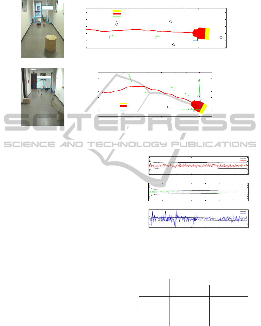
MARKERS

-1

-0.5

0.5

1.5

2 3 4 5 6 7 8 9 10 11 12

Building 1 (Pal1)

Warning Area

Protective Area

Mappa

Observation

Robot

Markers

(a) (b)

MARKERS

-2

-1.5

-1

-0.5

0.5

1.5

1 2 3 4 5 6 7 8 9 10

Building 3 Test B (Pal3b)

Warning Area

Protective Area

Map

Observation

Robot

Markers

Figure 4: Pictures of experimental environments in Building 1 (Pal1) (a) and Building 3 (Pal3 (c) and the respective polygonal

maps (b) and (d).

shown in the following are not signiﬁcantly differ-

ent from those achieved in other environments, even

without a speciﬁc ﬁlter for dynamic objects. Sim-

ulations have been performed using the MobileSim

simulator provided within the MobileRobots ARIA

library that introduces noise both to odometry and

range ﬁnder measurements, although not controlled

by the user. Real experiments have been executed on

a MobileRobots Pioneer 3DX equipped with a Sick

LMS100 laser scanner. Figures 4(a)-(c) illustrate the

real environments Pal1 and Pal3.

In each environment, the robot repeatedly moved

on a ﬁxed path consisting of the union of third or-

der splines. The length of the path is approximatively

9 − 12 m in each test run. Obstacles have been placed

so that, while the robot moves along its trajectory,

such objects partially or totally lie inside the warning

or the protective areas. The measurements collected

during the ﬁrst transit of the robot are used to build the

local map of each environment that is used as refer-

ence map for the successive acquisitions. During each

next transit, the robot extracts polylines from each

laser scan and associates them to the corresponding

polylines of the reference map according to the pro-

posed algorithm. The new polylines are not merged

into the reference map since the purpose of the ex-

periment is the assessment of the proposed represen-

tation. Figures 4(b)-(d) illustrate the polygonal maps

obtained in the experimental tests Pal1 and Pal3b.

In the simulation tests, the robot pose has been

estimated only by integrating odometry information

-0.01

-0.005

0.005

0.01

0 50 100 150 200 250 300 350

correzione x [m]

iterazioni

Deviazione standard x

Correzione x

-0.04

-0.03

-0.02

-0.01

0.01

0.02

0.03

0.04

0 50 100 150 200 250 300 350

correzione y [m]

iterazioni

Deviazione standard y

Correzione y

-0.015

-0.01

-0.005

0.005

0.01

0.015

0 50 100 150 200 250 300 350

correzione θ [rad]

iterazioni

Deviazione standard θ

Correzione θ

Figure 5: Corrections performed by the EKF localizer on

state variables x, y and θ during an experiment.

Table 1: Average, minimum and maximum restricted Haus-

dorff distances of the polylines w.r.t. reference maps within

the respective standard deviation for each simulated and real

environment.

Distance [cm]

Environment Mean Std Dev

Avg Min Max Avg Min Max

Sim1 4.71 2.19 6.62 1.89 1.25 2.69

Sim2 4.46 1.20 12.37 2.13 0.91 5.14

Pal1 2.46 1.78 2.86 1.09 0.99 1.16

Pal3a 3.99 2.14 5.94 1.68 0.70 3.18

Pal3b 4.55 2.88 6.86 1.72 1.21 3.45

due to the limitations of the simulator. In particular,

the simulated groundtruth is not directly accessible by

the application and the laser data do not include the

beam remission values making impossible to detect

reﬂective markers. Thus, the EKF localizer described

Semi-staticObjectDetectionusingPolygonalMapsforSafeNavigationofIndustrialRobots

197

in section 5 can be used only for tests in real environ-

ment. Figure 5 illustrates the trend of the correction

performed by the EKF ﬁlter on robot state variables x,

y and θ for a single test run in Pal1 within the corre-

sponding σ-bound computed from the covariance ma-

trix. The value of correction is bound by or compara-

ble to the σ-bound. Similar measures have been per-

formed in all the runs and for all the environments. In

all cases, the standard deviation is less than 6 mm for

position and 0.020 rad for angular variables.

The precision of the polygonal maps is measured

by the restricted Hausdorff distances between the cor-

responding polylines of the reference map and of cur-

rent observation. Table 1 reports the results for the

different environments. For each polyline i of the ref-

erence map, the mean restricted Hausdorff distance

and the corresponding standard deviations σ

have

been estimated. The results in the table are respec-

tively the average, minimum and maximum values of

mean distances µ

and standard deviations σ

for all

the polylines. The mean distance and variance in the

simulated environments are greater than in the real en-

vironments. This outcome can be explained with the

high accuracy achieved by the localizer. The overall

error is always less than 10 cm.

7 CONCLUSIONS

In this paper, we have presented a method to build

polygonal local maps that manage semi-static objects

in order to improve the navigation of industrial UGVs.

The maps consists of polylines extracted from laser

scans representing the boundary of objects. The pro-

posed methods extracts, associates and merges the

polylines obtained from the scan into a consistent

map. The proposed data association algorithm is

based on both the shape similarity measure and the re-

stricted Hausdorff distance, a novel metric proposed

in this work. The accurate environment reconstruc-

tion allows the identiﬁcation of semi-static objects

and the deﬁnition of efﬁcient navigation policies. To

replicate the navigation system of industrial UGVs,

an EKF localizer and a ﬁxed path navigation system

have been implemented. Experimental results show

that the error of the reconstruction is smaller than

10 cm. In our future works, we expect to exploit the

polygonal into a complete localization and mapping

algorithm.

ACKNOWLEDGEMENTS

This research is partially supported by SICK SPA.

REFERENCES

Arras, K. O. (2003). Feature-Based Robot Navigation

in Known and Unknown Environments. PhD the-

sis, Swiss Federal Institute of Technology Lausanne

(EPFL), Th

ese No. 2765.

Douglas, D. and Peuker, T. (1973). Algorithms for the re-

duction of the number of points required to represent

a digitized line or its caricature. Cartographica: Int.

Jour. for Geographic Information and Geovisualiza-

tion, 10(2):112–122.

Esteves, J. S., Carvalho, A., and Couto, C. (2003). Gen-

eralized geometric triangulation algorithm for mobile

robot absolute self-localization. In Proc. of IEEE

International Symposium On Industrial Electronics

(ISIE).

Fox, D., Burgard, W., and Thrun, S. (1999). Markov lo-

calization for mobile robots in dynamic environments.

Journal of Artiﬁcial Intelligence Research, 11:391–

427.

Katz, R., Douillard, B., Nieto, J., and Nebot, E. (2008). A

self-supervised architecture for moving obstacles clas-

siﬁcation. In Proc. of the IEEE/RSJ Int. Conf. on In-

telligent Robots and Systems (IROS).

Latecki, L. and Lakaemper, R. (1999). Convexity rule for

shape decomposition based on discrete contour evo-

lution. Computer Vision and Image Understanding,

73(3):441–454.

Latecki, L., Lakaemper, R., Sun, X., and Wolter, D. (2004).

Building polygonal maps from laser range data. In

ECAI Int. Cognitive Robotics Workshop.

Meyer-Delius, D., Hess, Grisetti, G., and Burgard, W.

(2010). Temporary maps for robust localization in

semi-static environments. In Proc. of the IEEE/RSJ

Int. Conf. on Intelligent Robots and Systems (IROS),

Taipei, Taiwan.

Morin, P. and Samson, C. (2008). Motion control of

wheeled mobile robots. In Siciliano, B. and Khatib,

O., editors, Springer Handbook of Robotics, pages

799–826. Springer Berlin Heidelberg.

Spinello, L., Triebel, R., and Siegwart, R. (2009). Multi-

class multimodal detection and tracking in urban en-

vironments. In Proc. of The 7th International Confer-

ence on Field and Service Robotics (FSR).

Stachniss, C. and Burgard, W. (2005). Mobile Robot Map-

ping and Localization in Non-Static Environments. In

Proc. of the National Conference on Artiﬁcial Intelli-

gence (AAAI).

Tipaldi, G. and Ramos, F. (2009). Motion clustering and

estimation with conditional random ﬁelds. In Proc. of

the IEEE/RSJ Int. Conf. on Intelligent Robots and Sys-

tems (IROS).

Wolf, D. and Sukhatme, G. (2005). Mobile robot simulta-

neous localization and mapping in dynamic environ-

ments. Journal of Autonomous Robots, 19:53–65.

Xavier, J., Pacheco, M., Castro, D., and Ruano, A. (2005).

Fast line, arc/circle and leg detection from laser

scan data in a player driver. In Proc. of the IEEE

Int. Conf. on Robotics & Automation (ICRA).

ICINCO2012-9thInternationalConferenceonInformaticsinControl,AutomationandRobotics

198