Efficient Distributed Fusion Filtering Algorithms
for Multiple Time Delayed Systems
Il Young Song and Moongu Jeon
School of Information & Communications, Gwangju Institute of Science and Technology
Oryong-Dong, Buk-Gu, 500-712, Gwangju, South Korea
Keywords: Distribute Fusion, Multi Sensor, Kalman Filter, Time-delayed System, Receding Horizon.
Abstract: In this paper, we provide two computational effective multi sensor fusion filtering algorithms for discrete-
time linear uncertain systems with state and observation time delays. The first algorithm is shaped by
algebraic forms for multi rate sensor systems, and then we propose a matrix form of filtering equations
using block matrices. The second algorithm is based on exact cross-covariance equations. These equations
are useful to compute matrix weights for fusion estimation in a multidimensional-multisensor environment.
Also, our proposed filtering algorithm is based on the receding horizon strategy in order to achieve high
estimation accuracy and stability under parametric uncertainties. We demonstrate the low computational
complexities of the proposed fusion filtering algorithm and how the proposed algorithm robust against
dynamic model uncertainties comparing with Kalman filter with time delays.
1 INTRODUCTION
In the past decades, state estimation problem for
dynamic systems with time delays has received a
great deal of research interest. The time delay
phenomenon in state variables is unavoidable in
many real systems (Anderson and Moore, 1979),
such as low earth orbit (LEO) satellite
communication systems (Glistic et al., 1996).
Ignorance of the computation of these delays could
cause unpredictable and unsatisfactory system
performance with traditional Kalman filters.
Using finite-memory estimation, we can obtain
an estimate based on data from the recent past only
(receding horizon). As a result, finite-memory filters
such as receding horizon Kalman filters are more
robust against model uncertainties and numerical
errors than standard Kalman filters, which utilize all
measurements (Kim et al., 2006 and Kim et al.,
2007). Thus, a receding horizon filter was chosen in
this study.
Based on aforementioned literature, and to the
best of the authors’ knowledge, there are no existing
results for the receding horizon filtering for linear
systems with time delays. Motivated by the above
problems, we focus on estimating the state of a
discrete-time linear system with time delays in both
the state and observation matrices, using a receding
horizon strategy. The main contribution of the paper
is to propose a fusion filtering algorithm using fusion
formulas for the systems with time-delays. Moreover,
a matrix form of filtering equations using block
matrices is also discussed, because this form is useful
to simply the filtering equations and derivation of
crucial Lyapunov-like equations for receding horizon
mean and covariance of systems with an arbitrary
number of time delays. Finally, the obtained results
are valid for general linear systems having time
delays in both dynamic and observation models.
The rest of this paper is organized as follows. In
Section II, the problem statement and description of
the Kalman filter with time delays (KFTD) are
given. In Section III, we present the receding
horizon filter for discrete-time linear systems with
time delays. Here, the exact recursive equations for
determining receding horizon initial conditions
(mean and covariance) are derived and discussed. In
Section IV, two computational effective multi sensor
fusion receding horizon filtering algorithms are
presented. To achieve the fusion filtering, local
cross-covariances are required. Thus, the equations
of the exact cross-covariance are derived using the
proposed form. In Section V, the effectiveness and
comparative analysis of the proposed filter with the
KFTD are then presented. Finally, a brief conclusion
is given in Section VI.
351
Young Song I. and Jeon M..
Efficient Distributed Fusion Filtering Algorithms for Multiple Time Delayed Systems.
DOI: 10.5220/0003970703510356
In Proceedings of the 9th International Conference on Informatics in Control, Automation and Robotics (ICINCO-2012), pages 351-356
ISBN: 978-989-8565-21-1
Copyright
c
 2012 SCITEPRESS (Science and Technology Publications, Lda.)

2 PROBLEM STATEMENT
The discrete-time linear uncertain systems with state
and observation time-delays considered in this paper
described by stochastic recursive equation with
time-delays,
≥
∑
M
h=0
x(k + 1) = F(k - h)x(k - h) + w(k), M 0, k = 0, 1, ...,
(1)
where
R∈
n
x(k)
is an unknown state and
R
×
∈
nn
F(k - h)
,
h = 0,1, , MK
are time-varying system
matrices. It is assumed that
(
)
00
x(-s) ~ N x , P
,
s = 0, 1, ,MK
are initial conditions and a systems noise
R∈
n
w(k)
is a zero-mean white Gaussian noise with
covariance
{
}
ks
cov w(k)w(s) = Q(k)δ
, and
ks
δ
is the
Kronecker function.
Suppose that the overall discrete measurement
are composed N measurement sub-vectors (local
sensors)
(1) (N)
y
(k)
y
(k),,K
, i.e.,
()()
R
R
,
∈
∈
⎡⎤
⎣⎦
≥
∑
TT
(i) (N)
m
L
m
i
(i) (i) (i) (i)
i
1N
d=0
T
i
Y = y (k) y (k) ,(k)
y (k) = H (k - d)x(k - d) + v (k), y (k) , L
0,
i=1, ,N m + +m =m,
L
KL
(2)
where
R∈
(i)
i
m
y(k)
represents the local i-th sensor
measurement,
R∈
(i)
m
i
v(k)
is the i-th measurement
matrix, and
R∈
m
(i)
i
v (k)
is a zero-mean white
Gaussian noise with covariance
{
}
(i) (i) (i)
ks
cov v (k)v (s) = R (k)δ
.
We also assume that the initial states
x(-s)
,
s = 0,1, , MK
, system noise
w(k)
, and measurement
errors
(i)
(k), i = 1, , Nv K
are mutually uncorrelated, i.e.,
{}
{
}
{}{ }
≠
(i)
(i) (i) (j)
cov x(-s), w(k) = 0 cov x(-s), v (k) = 0
cov w(k), v (k) = 0 cov v (k), v (k) = 0
s = 0, 1, ..., M; i, j = 1, ..., N; i j.
,,
,,
(3)
The main problem associated with such systems
(1) and (2) is to find the optimal (in mean square
sense) estimate of the unknown state based on the
overall receding horizon sensor measurements
k
k-Δ
Y
with receding horizon time intervals
i
Δ ,i=1, ,N,K
i.e.,
{
}
()
{}
1N
(i) (i) (i)
i
(1) (N)
[k -Δ [k -Δ
(i)
[k -Δ
k
k-Δ :k] :k]
:k] i i
=(k-Δ ), y , ..., y
.
Y = Y , ..., Y ,
Yy k-Δ +1 (k) ,
i = 1, ..., N
(4)
There are two multi sensor fusion filtering
algorithms. The first algorithm represents an optimal
filtering (OF) algorithm, i.e., a mean-square estimate
of a state vector using the overall measurement
vector
Y(k)
(2) is calculated by the optimal filtering
equations presented in Priemer and Vacroux (1969)
and Mishra and Rajamani (1975). However the OF
algorithm is computationally expensive and it
requires big memory sources, especially when the
number of sensors N >> 1.
On the other hand, the second multi sensor
algorithm is referred as fusion filtering (FF) which is
achieved by combining N local estimates based on
individual (local) sensor measurements
(i)
y
(k), i = 1, , NK
. The FF is suboptimal, but since
the FF has parallel structure, it can be effectively
adoptable for multisensory environment with the
following advantages such as increase data input
rates, simple fault detection, low computational
complexity, and so on.
Therefore, since the FF can be adoptable in a
multisensory environment, in this paper, the FF is
considered for the system (1) and (2). To derive the
FF, the local filtering estimates of a state vector based
on individual sensor measurements
(i)
y
(k)
are
required.
The KFTD’s equations for the system (1) and (2)
presented by Priemer and Vacroux (1969) and
Mishra and Rajamani (1975). Using KFTD’s
equations, we propose their receding horizon version
for estimation of state
x(k)
using overall receding
horizon measurements
k
k-Δ
Y
in (4). The details of the
new receding horizon Kalman filter with time-delays
are given in the next section.
3 LOCAL RECEDING HORIZON
KALMAN FILTER WITH
TIME-DELAYS
To find
(
)
ˆ
(i)
xk|k
based on receding horizon
measurements
(i)
[k-Δ :k]
i
Y we propose to use KFTD
equations on the receding horizon interval
[
]
∈
i
sk-Δ ,k
. We obtain
()( )
() () ( ) ( )
{}
ˆˆ
ˆ
..., ...
⎡⎤
⎢⎥
⎣⎦
∑
i
L
(i) (i)
m
d=0
(i) (i)
(i) (i)
ii ii i
x s-m|s =x s-m|s-1
+G s y s - H s-d x s-d|s-1 ,
s=k Δ ,k Δ +1, k; m=1,2, ,M , M =max M,L .
--
(5)
() ( )( )
ˆˆ
∑
M
h=0
(i) (i) (i)
x s|s-1 = F s-h-1 x s-h-1|s-1 .
(6)
() ( ) () () ( )( )
ˆ
ˆ
ˆ
⎡
⎤
⎢
⎥
⎣
⎦
∑
i
L
(i) (i)
0
d=0
(i) (i) (i) (i)
xs
|
s=x s
|
s-1 +G s
y
s - H s-d x s-d
|
s-1 ,
(7)
ICINCO2012-9thInternationalConferenceonInformaticsinControl,AutomationandRobotics
352

where the receding horizon filter gains
(
)
...
(i)
m
i
Gs,m=0,1,,M
and error auto-covariances
(
)
(
)
(
)
{
}
()()()
ˆ
≤
(ii) (i) (i)
12 1 2
(i) (i)
1112
Ps,s
|
s=cove s
|
s,e s
|
s,
es|s=xs-xs|s,s,s s.
(8)
are described by
() ( ) ( )
()
() ( ) ( ) ( )
()
⎡⎤
×
⎢⎥
⎣⎦
∑
∑
i
i
12
L
T
(i) (ii) (i)
m
d=0
-1
L
T
(i) (i) (ii) (i)
112 2
d,d=0
G s = P s-m,s-d|s-1 H s-d
R s + H s-d P s-d ,s-d |s-1 H s-d .
(9)
()( )
() ( ) ( )
∑
i
1
(ii) (ii)
12 12
L
(i) (i) (ii)
h2
d=0
P s-h ,s-h |s =P s-h ,s-h |s-1
-G s H s-d P s-d,s-h
|
s-1 ,
(10)
()()( )()()
∑
12
M
(ii) (ii) T
112 2
h,h=0
P s+1,s+1|s = F s-h P s-h ,s-h |s F s-h +Q s .
(11)
In contrast to KFTD filtering, the local receding
horizon Kalman filtering with time delay
(LRHKFTD) (5)-(11) needs to initialize (M+1)
receding horizon initial conditions at
i
s=k-Δ
which represent an unconditional means and
covariances, i.e.,
()()
{}
()
()()
{}
()
()
()
{}
()
ˆ
ˆ
ˆ
(i)
def
def
def
ii i ii ii
ii i ii ii
ii i i
xk-Δ -M +1k-Δ =E x k-Δ -M +1 = m k-Δ -M +1 ,
xk-Δ -M +2k-Δ =E x k-Δ -M +2 = m k-Δ -M +2 ,
....................................
xk-Δ +1 k-Δ =E x k-Δ +1 = m k-Δ +1 .
(12)
and
()
()()
{}
()
(ii)
def
12 1 2 12
12
i
ii i
Ph, hk-Δ = cov x h , x h = P h , h ,
h, h = k Δ M+1, , k Δ +1.
-- -K
(13)
Remark 1. The horizon initial means (12) are
described by
() ()()
...,
∑
M
h=0
i
m t + 1 = F t - h m t - h , t = 0, 1, 2, k Δ +1-
(14)
with initial conditions
() ( ) ( ) ( )
0
m 0 = m -1 = m -2 = ... = m -M = x .
(15)
Remark 2. The receding horizon initial covariances
(13) satisfy Lyapunov-like recursive equations
() ()( )()()
...
∑
12
M
(ii) (ii) T
1122
h,h=0
i
P t+1,t+1 = F t-h P t-h ,t-h F t-h +Q t ,
t = 0, 1, 2, , k Δ +1,
-
(16)
()()()
()
()()
<
<
∑
1
12
(ii) (ii)
(ii) (ii)
M
1 2 11 11 2
l=0
1t-h,t-h 1 2
T
12 21 1 2
P t-h +1,t-h +1 = F t-h -l P t-h -l ,t-h +1
+Q t-h δ ,kh kh,
P t-h ,t-h =P t-h ,t-h , t h t h
--
--
(17)
with initial conditions
(
)
... .
(ii) (ii)
0
12 12
P-s,-s=P,s,s=0,1,,M (18)
Derivation of Lyapunov-like equations for mean
and covariance (14)-(18) is given in Appendix.
4 TWO COMPUTATIONALLY
EFFICIENT MULTI SENSOR
FUSION ALGORITHMS
To apply the receding horizon Kalman filtering with
time delay (5)-(11) to the real computation with
MATLAB, using the repetition of (5)-(11) is less
effective than direct matrix multiplications because
the matrix operations, i.e., multiplications, divisions,
and inversions take many optimized computational
algorithms in MATLAB. Therefore, we change the
filtering equation (5)-(11) into a matrix form for the
computational benefits on MATLAB.
4.1 Matrix Form of Filtering Equations
The equations (5)-(11) can be represented by block
matrices. Let us assume the following block
matrices
()
(
)
{}
()
()
×
×
≤≤
<≤
≤≤
<≤
⎧
⎪
⎨
⎪
⎩
⎧
⎪
⎨
⎪
⎩
nn i i i
(i)
i
(i)
nn i i
=
=
M
M
Fs-h, 0 h M,
Fs-h
0,Mh ,M=maxM,L,
Hs-j,0jL,
Hs-j
0,L j
.
(19)
() ()
()
()
()
()
()
()
()
[]
()
()
()
()()
()
()
()
()
()
ˆ
ˆˆ ˆ
,
⎡⎤
⎣⎦
⎡⎤
⎣⎦
⎡⎤
⎣⎦
i
i
i
T
TT T
(i) (i) (i) (i)
i
i
(i) (i) (i) (i)
i
T
T
TT
(i) (i) (i) (i)
01 M
(ii) (ii)
(ii)
(ii) (ii)
X s|s = x s|s x s-1|s x s-M |s
s
s
s
s, s | s s, s - M | s
s|s
s-M,s|s
L,
F=F(s)F(s-1) Fs-M
H = H(s) H(s-1) H s-M ,
G = G (s) G (s) G (s)
PP
Ω =
PP
,
L
L
L
L
MO M
L
()
()
() ()
()()
()
RR
××
××
∈∈
⎡⎤
⎢⎥
⎢⎥
⎢⎥
⎣⎦
⎡⎤ ⎡ ⎤
⎣⎦ ⎣ ⎦
⎡⎤
⎣⎦
i ii
iii
ii
n nM+1 nM+1 nM+2
n nnM nM+1 nM+1 n
0jh jh0 i
s-M,s-M |s
,
A= I 0 , B= I 0 ,
Ω =P , P=P,j,h=1, ,M+1,K
(20)
where
n
I is an
×
nn
indent matrix,
×nn
0 is an
×nn
zero
matrix, and
(
)
(ii)
0
Ω 00 =Ω
.
Then, based on (5)-(11), the filtering
equations are rewritten using (19), (20):
EfficientDistributedFusionFilteringAlgorithmsforMultipleTimeDelayedSystems
353

()
()
()
()
() ()
()
() ()
() ( )
() () () ( )
ˆ
ˆ
ˆ
ˆ
ˆ
ˆ
⎡⎤
⎢⎥
⎣⎦
⎡⎤
⎢⎥
⎢⎥
⎣⎦
(i)
(i)
(i)
(ii)
T
(ii) T (ii)
T
(ii) T (ii)
(i) (i) (i) (i) (i) (i)
X s-1|s-1
Xs|s-1=
X s-1|s-1
s|s-1
s-1|s-1 s-1|s-1
s-1| s-1 s-1|s-1
Xs|s=Xs|s-1 s s sXs|s-1
F(s - 1)
B,
Ω
F(s - 1)Ω F(s-1)+Q(s-1) F(s-1)Ω
=B B
,
Ω F(s-1) Ω
+G y -H
() ( ) ()
()
() ( ) ()
()
()
()
()
() ()
()
()
⎡⎤
⎣⎦
⎡⎤
⎣⎦
i
-1
TT
(i) (ii) (i) (i) (ii) (i) (i)
(ii) (i) (i) (ii)
nM+1
ss|s-1s ss|s-1s s
s|s s s s|s-1
,
G=Ω HHΩ H+R,
Ω =I -G H Ω .
(21)
Finally, the local estimate
()
ˆ
(i)
xk|k
and error-
covariance
()
(ii)
Pk,k|k
at current time k are
described as
() ()
(
)()
ˆ
ˆ
(i) (i) (ii) (ii) T
x k|k = X k|k k,k|k k|kA,P =AΩ A.
(22)
Differently from (5)-(11), the local estimate
(
)
ˆ
(i)
xk
|
k
is directly calculated using (22). Moreover, (21) is
shaped like the Kalman filter as well as more simple
(5)-(11) on MATLAB.
4.2 Distributed Fusion Form of
Filtering Equations
Through (20)-(22) for
i=1, ,NK
, we obtain N
LRHKFTDs
(
)
(
)
ˆ
ˆ
(1) (N)
xk|k,,x k|kK
with the
corresponding local error-covariance
(
)
(11)
Pk,k
|
k
()
(NN)
,,P k,k
|
kK
. Then, the distributed fusion estimate
(
)
ˆ
FF
xk|k
is determined using the following fusion
formula presented by Shin et al. (2006).
() ()
ˆ
ˆ
∑∑
NN
FF (i) (i) (i)
n
i=1 i=1
x k |k = k|kC(k)x , C(k)=I,
(23)
where
...
(i)
C(k),i,
j
=1, ,N
is
×nn
matrix weights
which are defined as
()
[]
-1
T
T-1 T-1
eenn
C(k) = D P (k)D D P (k), D = I I ,K
(24)
where
[
]
{}
R
R
ˆ
×
×
∈
⎡⎤
∈
⎣⎦
≠
(1) (N) nnN
N
(ij) nN nN
e
i, j=1
(ij) (i) (j)
(i) (i)
C(k) = C (k), ,C (k) ,
P (k) = P (k, k k) ,
P (k, k k) = cov e (k k) , e (k k) ,
e (k k) = x(k) - x (k k) , i, j = 1, , N, i j.
K
K
(25)
In order to compute the matrix weights
...
(i)
C(k),i,
j
=1, ,N
, the local cross-covariances
(ij)
P(k,kk)
,
...i,
j
=1, ,N
,
≠i
j
are required. Derivation
of (23)-(25) is given in Shin et al. (2006). In the next
section, the effectiveness of the fusion filtering is
presented.
5 NUMERICAL EXAMPLE
In this section, an example for discrete-time
dynamic systems with parametric model uncertainty
is presented. We compare the accuracies and
implementation time between two fusion algorithms:
the first is OF algorithm (see section 4.1) and the
second is the FF algorithm (see section 4.2). The
example demonstrates the robustness and
effectiveness of our proposed LRHKFTD (5)-(11) in
terms of mean square errors (MSEs).
We now consider the following LEO satellite
communication system with multiple time delay and
uncertainty (Glistic et al., 1996). LEO satellite
channels impart severe spreading in delay and
Doppler on the transmitted signal. The state vector
represents the received signal level [dB].
() ()
(
)
() ()
(
)
() ()
()
()()
() () ( ) ( ) ()
⎧
⎪
⎨
⎪
⎩
12 3
xk+1=0.995+δ k x k + 0. 190 +δ kxk-1+0.107+δ kxk-2+wk,
y k =0.4x k +0.1x k-1 +0.4x k-2 +v k ,
(26)
where
(
)
(
)
(
)
wk ~N0,Qk
and
() ()
()
vk ~N0,Rk
are
uncorrelated white Gaussian system and
measurement noises, respectively,
(
)
2
Qk =0.02,
(
)
Rk =0.5.
The initial values are
(
)
(
)
(
)
(
)
x0~Nx0,P0 ,
(
)
x0=1
[dB] and
(
)
P0 =1;
(
)
(
)
(
)
(
)
{
}
123
δ k=δ k, δ k, δ k
are uncertain model parameters which is assumed to
satisfy
()
() () ()
⎧
≤≤≤∈
⎪
⎨
⎪
⎩
123 UI
δ k0.05,δ k0.1,δ k0.01,kT,
δ k=
0, otherwise ,
(27)
where
[
]
UI
T = 40; 60
is the uncertainty interval (UI).
The common receding horizon length
Δ
of the
LRHKFTDs is taken as
com
Δ =5
. Finally, two fusion
receding horizon filters: OF and FF with the
LRHKFTDs (5)-(11) and two fusion non-receding
horizon filters: OF and FF with KFTD for the
system model (26) with the uncertainty
()
δ k
which
takes the form (27) are compared.
We now present model (26) to show robustness of
the proposed RHKFTD against the uncertainty. All
simulations were evaluated in terms of MSEs of
1000 Monte Carlo runs. We compare the MSEs of
OF with KFTD (“OFKF”), FF with KFTD (“FFKF”),
OF with RHKFTD (“OFRHF”) and FF with
RHKFTD (“FFRHF”) with common receding
horizon length
com
Δ
, i.e.,
(A) OF with KFTD (“OFKF”):
() () ()
ˆ
⎡
⎤
⎣
⎦
2
OFKF OFKF
Pk,kk=Exk-xkk,
(B) FF with KFTD (“FFKF”):
ICINCO2012-9thInternationalConferenceonInformaticsinControl,AutomationandRobotics
354

FF
K
P
(C) O
F
OFS
W
Δ
com
P
(D) F
F
FFS
W
Δ
com
P
Our
p
aforeme
n
uncertai
n
that insi
horizon
good p
e
horizon
f
the OF
fi
FF versi
o
The e
s
clearly
c
figure
w
MSEs o
f
FFKF)
a
versions
differen
c
negligib
l
our pr
o
implem
e
delays.
6 C
O
In this
p
filter for
in both
t
equatio
n
systems
filtering
matrix
MATL
A
equatio
n
covaria
n
number
o
To
v
RHKFT
D
systems
implem
e
demons
t
filter in
p
roduce
require
m
()
⎡
⎣
K
F
k, k k = E
x
F
with RHKF
T
()
(
⎡
⎣
W
kk =E x
F
with RHKF
T
()
(
⎡
⎣
W
kk =E x
p
oint of int
e
n
tioned filter
s
n
ty interval
U
I
T
de of the UI
,
filters (OFR
H
e
rformance c
o
filters (OFK
F
fi
lters give m
o
o
ns. Howeve
r
s
timation acc
u
c
ompared thr
o
w
e observe t
h
f
the non-rece
a
re remarkabl
y
(OFRHF
a
c
es between
l
e outside of t
h
o
posed algo
r
e
ntations in a
O
NCLUS
I
p
aper we pr
o
discrete-tim
e
t
he state and
n
s shaped by
c
are define
d
equations in
t
form has
A
B. Also,
t
n
s for recedi
n
n
ce of a sy
s
o
f time delay
s
v
erify the e
f
D
, an exam
p
with param
e
e
nted. Throu
g
t
rated that th
terms of MS
E
good res
u
m
ents.
() (
ˆ
FFKF
x
k-x k
T
D (“OFRHF
(
) (
ˆ
OFSW
Δ
com
k-x k
k
T
D (“FFRHF
”
(
) (
ˆ
FFSW
Δ
com
k-x k
k
e
rest is the
b
s
, both inside
a
[]
I
= 40; 60
. I
n
,
the first pa
i
H
F and FF
R
o
mpared to
F
and FFKF).
A
o
re accurate e
s
r
, these differ
e
u
racy of the
fi
o
ugh MSEs
i
h
at within the
ding horizon
y
larger than
a
nd FFRHF
)
all OF an
d
h
e
[
UI
T = 40; 6
0
r
ithm is s
u
multisensory
I
ONS
o
pose a new
e
linear syste
m
obse
r
vation
m
c
lassical form
s
d
, and then
t
o the matrix
computatio
n
t
he Lyapun
o
n
g horizon
i
s
tem state
w
s
are derived.
f
fectiveness
p
le for discr
e
e
tric model u
n
g
h the impl
e
e robustness
E
s and the p
r
u
lts in real
-
)
⎤
⎦
2
k
,
”
):
)
⎤
⎦
2
com
k
, Δ =5
”
):
)
⎤
⎦
2
com
k
, Δ =5
b
ehaviour of
a
nd outside o
f
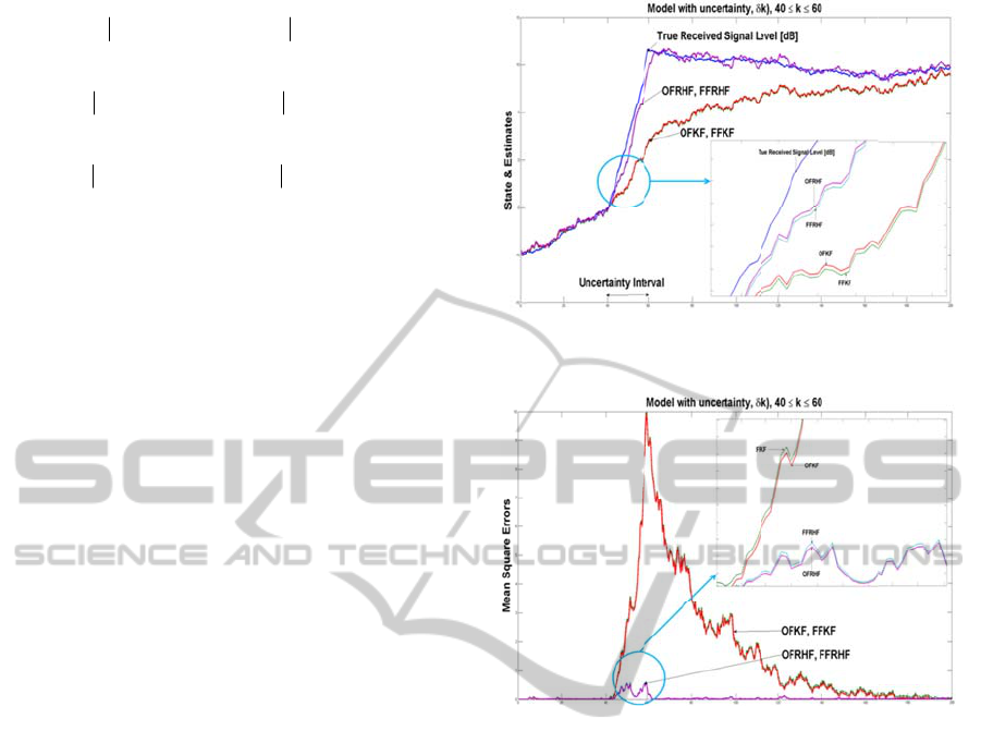
Fig.1 we obs
i
r of the rece
d
R
HF) demons
t
the non-rece
d
A
lso in each
p
s
timates than
t
e
nces are not
b
i
lters can be
m
i
n Fig. 2. I
n
[]
UI
T = 40; 60
,
f
ilters (OFKF
receding ho
r
)
. However,
d
FF filters
]
0
. For this re
a
u
itable for
system with
receding ho
r
m
with time d
e
m
atrices. Filt
e
s
for time-del
a
we change
form becaus
e
n
al benefits
o
v-like recu
r
i
nitial mean
w
ith an arbi
t
of the prop
o
e
te-time dyn
a
n
certainty
(
k
δ
e
mentations,
i
of the prop
o
r
opose
d
filter
-
time proce
s
,
.
f
the
f
the
s
erve
ding
t
rate
ding
p
air,
t
heir
b
ig.
m
o
r
e
n
the
,
the
F
and
r
izon
the
are
a
son,
real
time
r
izon
e
lays
e
ring
a
yed
the
e
the
on
r
sive
and
t
rary
o
sed
a
mic
)
k
is
i
t is
o
se
d
r
can
s
sing
Fig
u
OF
R
Fig
u
filt
e
filt
e
A
C
Th
i
Re
s
Fo
u
of
E
00
0
R
E
An
d
Gli
s
Ki
m
u
re 1: True rec
e
R
HF, FFRHF,
O
u
re 2: MSEs
e
rs (OFRHF a
n
e
rs (OFKF and
F
C
KNOW
L
i
s research
w
s
earch Progr
a
u
ndation of
K
E
ducation, S
c
0
4889).
E
FEREN
C
d
erson, B. D.
Filtering, Pren
s
tic, S., Talvit
e
(1996). Desig
n
network: do
w
J
ournal of Sel
e
1796–1808.
m
, D. Y., &
S
horizon FIR f
i
In Proceedin
g
e
ived signal le
v
O
FKF, and FF
K
c
omparison b
e
n
d FFRHF) a
n
F
FKF) with un
c
L
EDGEM
E
w
as support
e
a
m through t
h
K
orea (NRF)
fu
c
ience and T
e
C
ES
O., & Moore
t
ice-Hall.
e
, J., Kumpum
a
n
study for a C
D
n
link system
e
cted Topics in
S
hin, V. (200
6
lter fo
r
contin
u
gs
Inter. Conf.
v
el and its esti
m
K
F.
e
tween recedi
n
n
d non-recedi
n
n
certainty.
E
NTS
e
d by Basic
t
he National
f
unded by th
e
echnology (
N
, J. B. (1979
)
a
ki, T., & Lat
v
D
MA-
b
ased L
E
level parame
t
Signal Proces
s
6
). An optima
l
u
ous-time line
a
SICE-ICCAS
(
m
ates using
n
g horizon
n
g horizon
Science
Research
Ministry
N
o. 2011-
)
. Optimal
v
a-aho, M.
E
O satellite
ers, IEEE
s
ing, 14(9),
l
receding
a
r systems.
(
pp. 263–
EfficientDistributedFusionFilteringAlgorithmsforMultipleTimeDelayedSystems
355

265), Busan, Korea, Oct 2006.
Kim, D. Y., & Shin, V. (2007). Optimal receding horizon
filter for continuous time nonlinear stochastic systems.
In Proceedings of the 6
th
WSEAS Inter. Conf. on
Signal Processing (pp. 112–116), Dallas, Texas, USA,
Mar 2007.
Mishra, J., & Rajamani, V. S. (1975). Least-squares state
estimation in time-delay systems with colored
observation noise: an innovation approach, IEEE
Transactions on Automatic Control, 20(1), 140–142.
Priemer, R., & Vacroux, A. G. (1969). Estimation in linear
discrete systems with multiple time delays, IEEE
Transactions on Automatic Control, 14(4), 384–387.
Shin, V., Lee, Y., & Choi, T. (2006). Generalized
millman’s formula and its applications for estimation
problems, Signal Processing, 86(2), 257–266.
APPENDIX
Derivation of Equation for Receding Horizon
Initial Mean (14). Taking expectation on both sides
of (1) and using
(
)
[
]
Ewt =0
we immediately obtain
recursive equation (14) for mean
()
(
)
[
]
mt =Ext
.
Derivation of Equation for Receding Horizon
Initial Covariance (16). Subtracting (14) from (1)
we obtain time propagation of the centered state,
() ()()()
∑
M
h
h=0
x t+1 = F t-h x t-h +w t , t=0,1,2, ,
%%
K
(A.1)
Next we have
()() ( )( )( ) ( )()()
()()() ()()()
+
∑
∑∑
1
12
1 2
12
M
TTT
T
h
h1 1 2 2
2
h,h=0
MM
TT
T
h1 1 2h 2
h=0 h=0
x t+1 x t+1 = F t-h x t-h x t-h F t-h +w t w t
F t-h x t-h w t + w t x t-h F t-h .
%% % %
%%
(A.2)
Taking expectation on both sides of (A.2) and using
the fact that current noise
(
)
wt
does not depend on
current and past states
(
)( )
12
xt-h , xt-h
%%
we obtain
recursive equation for covariance (16),
() ()( )()()
∑
12
12
M
T
h1 12h 2
h,h=0
P t+1,t+1 = F t-h P t-h ,t-h F t-h +Q t .
(A.3)
Note that equation (A.3) contains auto-covariance,
()()()
()()()
⎡
⎤
⎣
⎦
T
12 1 2
12
P t-h ,t-h = E x t-h x t-h ,
x t-h = x t-h -m t-h ,
h , h = 0,1, , M.
%%
%
K
(A.4)
Derivation of Equation for Auto-covariance (17).
Using “symmetric” property of auto-covariance
()()
T
21 12
P t-h ,t-h = P t-h ,t-h and without loss of
generality we can assume that
≥
2
1
k-h k-h
.
Substituting
→
1
tt-h
in (A.1) we obtain
() ()()()
∑
1
1
M
1 l 11 11 1
l=0
xt-h+1= F t-h-l xt-h-l +wt-h .
%%
(A.5)
Multiplying both sides of (A.5) by
()
T
2
xt-h +1
%
and
using (A.4) we obtain
()() ()()()
()( )
∑
1
1
M
TT
12 l11112
l=0
T
12
x t-h +1 x t-h +1 = F t-h -l x t-h -l x t-h +1
+w t-h x t-h +1 ,
%% %%
%
(A.6)
and
()()()
()( )
⎡⎤
⎣⎦
∑
1
1
M
12 l11112
l=0
T
12 12
P t -h +1,t -h +1 = F t -h -l P t-h -l ,t -h +1
+E w t-h x t-h +1 , h ,h =0,1,. ,M.
%
K
(A.7)
It’s remain to calculate expectation in (A.7), i.e.,
()( )
for ≥⎡⎤
⎣⎦
T
12 12
E w t-h x t-h +1 t-h t-h .
%
(A.8)
Calculating product
()( )
T
12
w t-h x t-h +1
%
using (A.5)
and after that taking expectation we get
()( ) ()( ) ( )
()()
⎡⎤⎡⎤
⎣⎦⎣⎦
⎡⎤
⎣⎦
∑
2
M
TT
T
l
12 122 22
2
l=0
T
12
E w t-h x t-h +1 = E w t-h x t-h -l F t-h -l
+Ewt-h wt-h .
%%
(A.9)
According to assumption
≥
12
t-h t-h
, “future” noise
(
)
1
wt-h
does not depend on current and past states
(
)
22
xt-h -l
%
therefore
()( )
⎡⎤
⎣⎦
T
122
E w t-h x t-h -l =0.
%
Next using property of white noise we obtain
()() ()
⎡⎤
⎣⎦
12
T
12 1t-h,t-h
E w t-h w t-h =Q t-h δ .
(A.10)
Finally using (A.7), (A.9) and (A.10) we get
equation for auto-covariance (17).
This completes the derivation Lyapunov-like
equations for receding horizon mean and
covariances.
ICINCO2012-9thInternationalConferenceonInformaticsinControl,AutomationandRobotics
356