STATISTICAL ASYMMETRY-BASED BRAIN TUMOR
SEGMENTATION FROM 3D MR IMAGES
Chen-Ping Yu
1
, Guilherme C. S. Ruppert
2,3
, Dan T. D. Nguyen
4
, Alexandre X. Falcao
2
and Yanxi Liu
1
1
Department of Computer Science and Engineering, Pennsylvania State University
342 Information Sc. and Tech. Building, University Park, 16802 PA, U.S.A.
2
Institute of Computing, University of Campinas, Av. Albert Einstein 1251, 13083-852 Campinas, Brazil
3
Renato Archer Center for Information Technology, Rod. Dom Pedro km143, 13069-901 Campinas, Brazil
4
Department of Radiology, Penn State Hershey Medical Center, 500 University Drive, Hershey, 17033 PA, U.S.A.
Keywords:
Brain Tumor Segmentation, Brain Image Analysis, Computer Aided Diagnosis, Computational Symmetry,
MRI Analysis.
Abstract:
The precise segmentation of brain tumors from MR images is necessary for surgical planning. However, it
is a tedious task for the medical professionals to process manually. The performance of supervised machine
learning techniques for automatic tumor segmentation is time consuming and very dependent on the type
of the training samples. Brain tumors are statistically asymmetrical blobs with respect to the mid-sagittal
plane (MSP) in the brain and we present an asymmetry-based, novel, fast, fully-automatic and unsupervised
framework for 3D brain tumor segmentation from MR images. Our approach detects asymmetrical intensity
deviation of brain tissues in 4 stages: (1) automatic MSP extraction, (2) asymmetrical slice extraction for an
estimated tumor location, (3) region of interest localization, and (4) 3D tumor volume delineation using a
watershed method. The method has been validated on 17 clinical MR volumes with a 71.23%±27.68% mean
Jaccard Coefficient.
1 INTRODUCTION
Brain tumors vary in size, shape, color, and location,
which is precisely the reason why automatic tumor
segmentation is challenging. While the medical pro-
fessionals are able to hand label the optimal details
of each tumor case, such task is incredibly tedious
and time-consuming. Therefore, the need for tumors
to be automatically segmented remains an unsolved
problem in clinical practice.
In recent years, related unsupervised approaches
that utilizes brain asymmetry (Ray et al., 2007) (Joshi
et al., 2003) requires human interaction to manually
select a 2D slice of interest, and the 2D/3D tumor seg-
mentation from such analysis has not been shown to
work fully automatically.
Markov Random Fields (Li, 2001) and Condi-
tional Random Field (Lafferty et al., 2001) based ma-
chine learning techniques have been applied in tumor
segmentation tasks as well. Methods like Discrimina-
tive Random Fields (Kumar and Hebert, 2003), Sup-
port Vector Random Fields (Lee et al., 2005), and
Pseudo-Conditional Random Field (Lee et al., 2008)
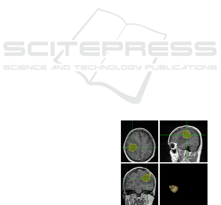
Figure 1: Sample result for case 6, showing the 3 orien-
tations and the 3D view on the lower right portion of the
figure, with Jaccard Coefficient of 90.11%.
have been shown to offer better performance. Other
supervised statistical machine learning approaches
include using fractal features (Iftekharuddin et al.,
2008), alignment features (Schmidt et al., 2005), one-
527
Yu C., C. S. Ruppert G., T. D. Nguyen D., X. Falcão A. and Liu Y..
STATISTICAL ASYMMETRY-BASED BRAIN TUMOR SEGMENTATION FROM 3D MR IMAGES.
DOI: 10.5220/0003892205270533
In Proceedings of the International Conference on Bio-inspired Systems and Signal Processing (MIAD-2012), pages 527-533
ISBN: 978-989-8425-89-8
Copyright
c
 2012 SCITEPRESS (Science and Technology Publications, Lda.)

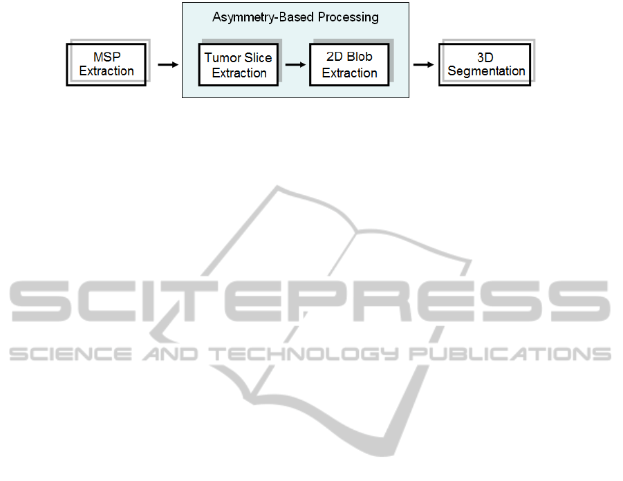
Figure 2: Diagram of the entire process of the proposed 4-stage algorithm.
class support vector machine (Zhang et al., 2004),
using Bayesian classifier (Corso et al., 2006), tumor
localization using diagonal nearest-neighbors (Ger-
ing, 2003), segmentation by outliers (Prastawa et al.,
2004), and high-dimensional features with level-set
(Cobzas et al., 2007). A recent supervised method
proposed (Koshy et al., 2011), though demonstrat-
ing promising results on small tumor detection using
brain asymmetry, is not addressing 3D tumor segmen-
tation problem.
In order to extract features to be used for
pixel/voxel classification, standard machine learning
methods must first register the input volume. The reg-
istration process usually takes hours of time while be-
ing a research area of its own (Klein et al., 2009); the
performance accuracy of the classification and seg-
mentation result depends largely on the training sam-
ples and the pre-defined feature sets.
Unsupervised algorithms using the bilateral sym-
metry of the brain start to emerge in recent years
(Mancas et al., 2005)(Ray et al., 2007). However, un-
supervised methods based on symmetry are still in its
early stages as such methods are not yet fully auto-
matic, and the accuracy also has a lot of room for im-
provements (Mancas et al., 2005)(Ray et al., 2007).
In this paper, we present a novel, fully automatic
and unsupervised framework that is based upon an
intuitive yet statistically justified observation that tu-
mors are one of the most prominent asymmetrical
blobs in the brain. We show that our approach is in-
variant to different types of tumor with the asymmet-
rical blob assumption, and we are able to automat-
ically localize and delineate the tumors. The entire
process is fast due to the unsupervised nature, taking
about 3 minutes to run.
2 STATISTICAL
ASYMMETRY-BASED
METHOD
Human brains are commonly accepted as statistically
symmetrical with respect to its Mid-Sagittal Plane
(MSP)(Ruppert et al., 2011). Our proposed method
takes the advantage of this property by processing the
brain through asymmetry comparisons of its struc-
tural and pixel intensity distribution. We propose a
4-stage process: 1) MSP alignment, 2) locate an ax-
ial slice that contains parts of the tumor, 3) localize
the 2D shape of the tumor from the extracted slice-of-
interest (SOI), 4) grow the 3D shape of the tumor out
bi-directionally.
2.1 Stage 1: Automatic Mid-Saggital
Plane Extraction
Since this work is a symmetry-based method, it de-
pends on the bi-lateral symmetry analysis of the brain,
which requires the localization of the mid-sagittal
plane (MSP) which is the reference of symmetry of
the brain. Based on the MSP location, the image can
be realigned, i.e. rotated and translated in a way so
the MSP is found in the central slice of the image.
In order to perform the MSP extraction, first, all in-
put images were re-interpolated to isotropic voxels to
restore the original proportion of the brain.
The method described in (Ruppert et al., 2011)
was used to automatically locate the mid-sagittal
plane (MSP). It is a very fast and accurate method
for MSP extraction and is based on bi-lateral symme-
try maximization. It uses cross-correlation of edges in
the full 3D domain as the symmetry criteria and finds
the plane that maximizes this criteria using an opti-
mized multi-scale search algorithm. On average, the
method takes less than 25s to run on a modern desk-
top machine over a typical MRI data. Figure 3 shows
some examples of the results from this method.
2.2 Stage 2: Slice of Interest (SOI)
Extraction
We formulate the problem using a Bayesian model,
P(Z|S
Z
) ∝ P(S
Z
|Z) × P(Z) (1)
Our goal is to extract a 2D slice E[S] from the vol-
ume of interest (VOI) that contains part of the tumor,
where we obtain E[S] from the posterior P(Z|S
Z
) by
maximizing the conditional likelihood P(S
Z
|Z). We
define S
Z
as the full count of axial-view slices from
the neck towards the top of the head, where S
Z
=
BIOSIGNALS 2012 - International Conference on Bio-inspired Systems and Signal Processing
528

Figure 3: Examples of results from Stage 1 (MSP extrac-
tion). The Figure shows 4 pairs (original image and the
results from the method) for cases 1, 3, 4 and 10 with slice
184, 160, 161, and 156 respectively.
{ S
L|Z
, S
R|Z
| Z = 1,...,z,L = l
1
,...,l
u
,R = r
1
,...,r
u
},
and a prior P(Z) that models the likelihood of tumor
location.
The brain is split into 2 halves along MSP of S
Z
,
where S
L|Z
and S
R|Z
are the left and right half. S
L|Z
and S
R|Z
are then further equally partitioned perpen-
dicular to the MSP into u pieces for the consideration
of spatial information.
We compute an asymmetry score using Earth-
Mover Distance (Ling and Okada, 2007) for each
pair of S
L|Z
and S
R|Z
that is equally partitioned into u
pieces. The Earth-Mover Distance between two nor-
malized histograms H(A) and H(B) is denoted here
as Φ( H(A), H(B) ). The normalized 3-dimensional
histogram (x,y location and the intensity level at
each pixel) of each partitioned piece are denoted as
H
3
(S
l
u
|Z
) and H
3
(S
r
u
|Z
). To determine how asymmet-
rically distributed are the intensity values of S
z
with
its piece-wise spatial information, each pair of parti-
tions’ EMD asymmetry scores are summed to form
the likelihood probability:
P(S
Z
) =
u
∑
i=1
Φ( H
3
(S
l
u
|Z
), H
3
(S
r
u
|Z
) ) (2)
We obtain the likelihood probability from each
slice S
z
, which we can plot and treat as a 1D signal
(Figure 4). We wish to locate the most asymmetri-
cal slice. However, this signal can be noisy due to
different parts of the brain (especially the neck region
and the scalp top) and intensity variance, therefore we
must apply a prior P(Z) that models the likelihood of
tumor location. We found that parts of the Inverse-
Gamma distribution resembles the prior likelihood of
tumor location well (Figure 4). We denote Inverse-
Gamma as f (Z;α, β), and it is defined as:
P(Z) = f (Z; α,β) =
β
α
Γ(α)
(1/Z)
α+1
e
−β/Z
(3)
The Inverse-Gamma prior formulates the likeli-
hood P(S
Z
) into a conditional probability P(S
Z
|Z).
Now we can calculate Bayesian posterior probability
P(Z|S
Z
) from the originally obtained conditional like-
lihood signal P(S
Z
|Z) with the Inverse-Gamma prior
P(Z).
After P(Z|S
Z
) is computed, any posterior prob-
ability that is outside of 3σ is reduced to the mean
of the entire posterior probability and its S
Z−2
, S
Z−1
,
S
Z+1
, and S
Z+2
neighbors as a measure to remove out-
liers. The processed posterior probability P(Z|S
Z
) is
convoluted by 1D Gaussian filter N(µ = 0,σ
2
= 3)
with horizontal size of 9 (spans 4 slices before and
after the current position) for all observations to be
weighted by their neighboring information as well as
filtering out the high frequency noises (Figure 4). Fi-
nally we can take the maxima of this signal to be our
E[S] and proceed to segment tumor’s 2D shape (Fig-
ure 4). We define the convulotion of f and g as f ?
g, and by setting the parameters Z = 1 : z, µ = 0, and
σ = 3, we are able to find the tumor slice:
E[S] = max{ P(Z|S
Z
) ? N(µ,σ) } (4)
2.3 Stage 3: Blob Feature Extraction
with Asymmetry Processing
From the extracted slice of interest, we proceed to ex-
tract the tumor’s 2D shape with a state of the art blob
detector. We use Center-Surround Distribution Dis-
tance (CSDD) (Collins and Ge, 2008) as our blob and
interest region detector, which is insensitive to geo-
metric deformation. CSDD is based on comparing
the cumulative distributions of intensity and texture of
an extracted region and its surrounding circular back-
ground.
E[S] is first smoothed with Gaussian low-pass fil-
ter, where N(l = 5,µ = 0, σ
2
= 2) to get rid of possi-
ble noise, then CSDD blob features (Collins and Ge,
2008) are extracted from the filtered E[S] (Figure 5).
We denote the extracted blob features as
→
B
with each
single blob feature denoted as B
i
. To eliminate all the
false positives blobs that do not surround the actual tu-
mor, we compute the EMD (Ling and Okada, 2007) of
the intensity distribution 1D histogram (only intensity
information) from the areas enclosed by each blob B
i
and its corresponding MSP-reflection area Re f (B
i
),
and retain the highest 5% EMD metric blobs, denoted
as
→
B
∗
, in which blobs with higher EMD score imply
the enclosed structure as being more asymmetrical.
→
B
∗
= max{ Φ( H
1
(B
i
), H
1
(Re f (B
i
)) ),

5N
100

} (5)
We define and compute the tumor-likelihood score
STATISTICAL ASYMMETRY-BASED BRAIN TUMOR SEGMENTATION FROM 3D MR IMAGES
529

Figure 4: The complete process of Slice of Interest E[S] extraction: (a) Inverse-Gamma prior P(Z), (b) spatially-constrained
EMD asymmetry distance for S
Z
, (c) posterior probability P(Z|S
Z
), (d) P(Z|S
Z
) is filtered by Gaussian low-pass filter with
σ = 3, (e) the most asymmetrical slice E[S] extracted as the maxima of P(Z|S
Z
).
Figure 5: Case #1 intermediate results for tumor blob detection: (a) E[S], (b) extracted CSDD blob features
→
B
, (c) the top 5%
most asymmetrical blobs
→
B
∗
the whiter the outline represents the higher asymmetrical score, with the extracted MSP as the
white vertical line, (d) result of k-means clustering with y-axis as the tumor-likelihood P(B
∗
j
) for each blob B
∗
j
, (e) retaining
the cluster that yields the higher mean P(B
∗
j
) gives us the true positive tumor blobs E[
→
B
∗
], (f) the final 2D rough tumor shape.
P(B
∗
j
) of each blobs B
∗
j
of
→
B
∗
by weighting EMD
asymmetry score of B
∗
j
with its blob strength S(B
∗
j
),
which is the EMD measure of how distinctive is
the foreground and background intensity of blob B
∗
j
.
Then, we dividing the weighted asymmetry score by
its foreground intensity variance Var[I(B
∗
j
)], because
the non-tumor false positives such as part of the scalp
and surrounding tissues may yield high intensity vari-
ance, whereas the tumor tissue in an area remains uni-
form intensity.
P(B
∗
j
) =
S(B
∗
j
) Φ( H
1
(B
∗
j
), H
1
( Re f (B
∗
j
) ) )
Var[ I(B
∗
j
) ]
(6)
K-means clustering (Alsabti et al., 1998) algo-
rithm with k = 2 is then used to cluster P(
→
B
∗
) into
two groups
→
B
∗
k=1
and
→
B
∗
k=2
, and the expected tumor
blobs E[
→
B
∗
] can be retained by keeping the cluster that
yields the highest likelihood (Figure 5).
E[
→
B
∗
] = max{ avg(
→
B
∗
k=1
), avg(
→
B
∗
k=2
) } (7)
It is possible that E[
→
B
∗
] can have blobs at spur and
false positive locations instead of one connected com-
ponent. In which case, we use a heuristic approach to
remove outlier blobs by keeping the connected com-
ponent that has the most blobs with the highest EMD
asymmetry score Φ( H
1
(B
∗
j
), H
1
( Re f (B
∗
j
) ). To ob-
tain the final rough 2D location and shape of the tu-
mor from E[
→
B
∗
], simply segment the combined con-
tour of the blobs E[
→
B
∗
], which yields the rough 2D
shape of the tumor (Figure 5).
2.4 Stage 4: 3D Tumor Delineation by
IFT (Image Forest Transform)
Watershed
The previous steps provide the approximate location
of the tumor and a rough shape of this tumor within
the SOI. The next step is the precise delineation of the
tumor and this is performed for the whole 3D image.
The approach we use in this work utilizes
markers-controlled watershed, placing object and
background seeds within the SOI and letting the wa-
tershed (Grau et al., 2004) grow the regions in 3D.
However, there are many different algorithms of wa-
tershed and their segmentation results are not the
same (Audigier and Lotufo, 2007). In this work,
we use the IFT-watershed (Lotufo and Falcao, 2000)
which is based on the Image Foresting Transform
(Lotufo and Falcao, 2000). IFT is a general tool
for designing of image processing operators based
on connectivity, reducing image processing problems
into an optimum path forest problem in a graph de-
rived from the image. We chose the IFT-watershed
BIOSIGNALS 2012 - International Conference on Bio-inspired Systems and Signal Processing
530

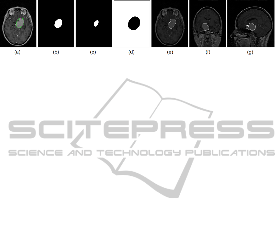
Figure 6: IFT-Watershed segmentation process and result. (a) input image, (b) initial mask, (c) tumor seeds, (d) background
seeds, (e)-(f) final segmentation in axial, coronal and sagittal orientation, respectively.
method because it is considerably faster (Lotufo and
Falcao, 2000) and implements the watershed in such
a way that resolves the ”tie zones” dividing them in
a balanced manner between the seeds. Further infor-
mation about the details and evaluation of the IFT-
Watershed can be found in (Audigier and Lotufo,
2007) and (Lotufo and Falcao, 2000).
However, the watershed requires an initialization
by placing some object and background seeds, so we
developed a way to automatically place these seeds
using the result from the blobs extraction stage. In
our case, the term ”object” below refers to the tumor,
and the background refers to everything else.
The result from the blob extraction is a 2D binary
mask (where we have zero for background and one
for object). To generate the object seeds, we apply
the erosion morphological operator on this mask us-
ing a circular structuring element with radius adaptive
to the input mask. This morphological operation is
performed in 2D within the SOI. The result is shown
in Table 6. The background seeds are generated in a
similar way by applying the dilation operator instead
of erosion but then computing the complement of the
image (inverting values 0 for 1 and vice-versa), result-
ing in the image shown in Table 6.
In essence, we create a region of uncertainty
around the borders of the mask within the SOI. By
definition, the internal seed voxels are already con-
sidered to be tumor voxels, and the background seeds
are non-tumor voxels. The unmarked voxels are the
region of uncertainty which will be resolved by the
IFT-Watershed.
Although the seed generation is performed only
in one slice (SOI), we let the watershed grow to the
rest of the 3D image. Figure 6 shows the resulting
segmentation after the IFT-Watershed.
3 RESULTS
We test our algorithm on 17 MRI data. The 17 3D
MR volumes are T1 weighted and post gadolinium
enhanced images acquired in the Axial plane. Other
modalities such as T2 or FLAIR are not required by
our proposed method.
By visual inspection, the MSP alignments (stage
1) are sucessful for all 17 brain scans in the
dataset,which is critical to the success of our symme-
try based algorithm. Stage 2 (SOI extraction) located
correct slices for 14 out of 17 cases, where stage 3 (2D
localization) located the correct tumor location in 13
of 14. Stage 4 (IFT-Watershed) was able to segment
the 3D shape of the tumor in all 13 with 1 of which
that was not as good due to complicated tumor tissue.
Overall, our stage 3 and stage 4 generates very ro-
bust results based on the slice that was extracted from
stage 2.
Quantitative results are calculated using Jaccard
Coefficient, where the True Positives (TP) are identi-
fied as the overlap between the manually segmented
ground truth tumor labels and the machine generated
tumor labels.
Jaccard Coefficient:
JC =
T P
FP + FN + T P
(8)
Our proposed algorithm achieves the mean Jac-
card Coefficient of 71.23% ± 27.68% and the median
of 81.68% from the cases that produced outputs. If
we disregard case 17 where it failed miserably and
should be considered as a failure case, our mean Jac-
card Coefficient is in fact 77.11% ± 18.57%. We also
visually inspect the output of each intermediate stages
and label the result as either Match and Mismatch to
indicate whether or not the tumor has been located.
To further demonstrate the robustness of the blob lo-
calization (stage 3) asymmetry processing, we man-
ually select a tumor slice if stage 2 fails to locate a
tumor slice (case 10, 12, and 15) and shows very high
accuracy. Table 2 shows the complete quantitative re-
sults where bold letters indicate manual selected tu-
mor slice in the case of failed stage 2.
Comparing to other unsupervised and symmetry-
based methods (Mancas et al., 2005)(Ray et al.,
2007), our proposed method is able to work fully au-
tomatically without any user intervention, and is pro-
cessed fully in 3D. We also achieve a much higher
STATISTICAL ASYMMETRY-BASED BRAIN TUMOR SEGMENTATION FROM 3D MR IMAGES
531

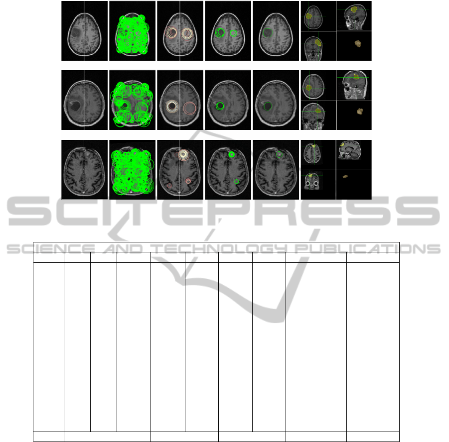
Figure 7: Sample Results. Row 1 to 3: Case 5, 6, and 11.
Table 1: Results for the 4-Stage on all 17 Cases.
Post MSP Extraction 3-Stage Result for 17 Cases
Case # Stg 1 Stg 2 time (s) Stg 3 time (s) Stg 4 time (s) Total run-time (s) Jcrd Coeff (%)
1 1.47 In 108.44 Auto 48.48 Success 40.28 197.2 93.99
2 0.85 In 104.35 Auto 76.34 Success 43.17 223.86 88.07
3 2.47 In 114.24 Auto 81.03 Success 42.61 237.88 73.92
4 2.76 In 111.36 Auto 79.23 Success 38.01 228.6 72.61
5 2.10 In 98.02 Auto 65.12 Success 42.35 205.49 81.68
6 3.08 In 113.25 Auto 79.21 Success 38.55 231.01 90.11
7 1.97 In 94.55 Auto 69.49 Success 35.29 199.33 31.74
8 1.14 In 106.41 Auto 73.88 Success 44.78 225.07 54.10
9 1.15 In 51.57 Auto 42.51 Success 26.42 120.50 92.61
10 1.39 Out 61.74 Manual 51.66 Success 34.21 147.61 87.47
11 1.02 In 42.66 Auto 47.60 Success 19.34 109.6 69.85
12 1.29 Out 44.93 Manual 62.97 Success 29.05 136.95 90.57
13 0.37 In 55.89 Auto 57.90 Success 26.93 140.72 92.66
14 1.23 In 104.53 Auto 88.29 Success 36.18 229.00 83.98
15 0.97 Out 30.35 Manual 62.81 Success 13.59 106.75 90.73
16 1.49 In 33.03 Auto 57.23 Fail 20.31 110.57 0.00
17 0.47 In 68.6 Auto 74.67 Fail 24.89 168.16 0.61
Mean 79.06±31.26 65.79±13.45 32.70±9.46 177.55±49.47 71.23±27.68
accuracy than what’s reported from (Ray et al., 2007)
(highest segmentation score being 71.15%), with very
fast mean run time of under 3 minutes per 3D MR
scan, which is very fast comparing to recent publi-
cations in both supervised and unsupervised related
work.
4 CONCLUSIONS
We have proposed a novel unsupervised statisti-
cal asymmetry-based, automatic tumor segmentation
framework. The method combines a set of state of the
art computer vision techniques and has been validated
on 17 clinical MR images. Our future work will focus
on developing robust segmentation methods for more
challenging cases where small, multiple tumors, and
diffused boundaries are present.
REFERENCES
Audigier, R., Lotufo, R. A. (2007). Watershed by Image
Foresting Transform, Tie-Zone, and Theoretical Rela-
tionships with Other Watershed Definitions. In: Pro-
ceedings of the 8th International Symposium on Math-
ematical Morphology
Alsabti, K., Ranka, S., Singh, V. (1998). An efficient k-
BIOSIGNALS 2012 - International Conference on Bio-inspired Systems and Signal Processing
532

means clustering algorithm. In: Proc. 1st Workshop
on High Performance Data Mining
Cobzas, D., Birkbeck, N., Schmidt, M., Jagersand, M.,
Murtha, A. (2007). 3D Variational Brain Tumor
Segmentation using a High Dimensional Feature Set.
ICCV
Collins, R., Ge, W. (2008). CSDD Features: Center-
Surround Distribution Distance for Feature Extraction
and Matching. ECCV
Corso, J. J., Sharon, E., Yuille, A. (2006). Multilevel Seg-
mentation and Integrated Bayesian Model Classifica-
tion with an Application to Brain Tumor Segmenta-
tion. MICCAI
Bergo, F. P., Falcao, A., Yasuda, C., Ruppert, G. (2008).
Fast and Robust Mid-Sagittal Plane Location in 3D Mr
Images of the Brain: Biomedical Engineering Systems
and Technologies, vol. 25, pp. 278-290
Gering, D. T. (2003). Diagonalized nearest neighbor pattern
matching for brain tumor segmentation. MICCAI
Grau, V., Mewes, A. U. J., Alcaniz, M., Kiminis, R.,
Warfield, S. K. (2004). Improved watershed transform
for medical image segmentation using prior informa-
tion. IEEE Transactions on Medical Imaging, vol. 23,
iss. 4
Iftekharuddin, K. M., Zheng, J., Islam, M. A., Ogg, R. J.
(2008). Fractal-based brain tumor detection in multi-
modal MRI. AMC
Joshi, S., Lorenzen, P., Gerig, G., Bullitt, E. (2003). Struc-
tural and radiometric asymmetry in brain images.
Medical Image Analysis, 7(2): 155-170
Klein, A., Andersson, J., Ardekani B. A., Ashburner J.,
Avants B., Chiang M. C., Christensen G. E., Collins
D. L., Gee J., Hellier P., Song J. H., Jenkinson M.,
Lepage C., Rueckert D., Thompson P., Vercauteren T.,
Woods R. P., Mann J. J., Parsey R. V. (2009). Evalu-
ation of 14 non-linear deformation algorithm applied
to human brain MRI registration. Neuroimage
Kumar, S., Hebert, M. (2003) Discriminative fields
for modeling spatial dependencies in natural images.
NIPS
Lafferty, J., Pereira, F., McCallum, A. (2001). Conditional
random fields: Probabilistic models for segmenting
and labeling sequence data. ICML
Lee, C.H., Greiner, R., Schmidt, M. (2005). Support vector
random fields for spatial classification. In: PKDD, pp.
121–132
Lee, C. H., Wang, S., Murtha, A., Brown, M. R. G., Greiner,
R. (2008). Segmenting Brain Tumors using Pseudo-
Conditional Random Fields. MICCAI
Li, S. Z. (2001). Markov Random Field Modeling in Image
Analysis. Springer-Verlag, Tokyo
Mancas, M., Gosselin, B., and Macq,B. (2005). Fast and
automatic tumoral area localization using symmetry.
IEEE International Conference on Acoustics, Speech
and Signal Processing, 2: 725-728
Ling, H., Okada, K. (2007). An Efficient Earth Mover’s
Distance Algorithm for Robust Histogram Compari-
son. PAMI
Lotufo, R., Falcao, A. (2000). The ordered queue and the
optimality of the watershed approaches, In: Math-
ematical Morphology and its Applications to Image
and Signal Processing, vol. 18, pp. 341-350
Ray, N., Saha, B., and Brown, M.(2007). Locating Brain
Tumors from MR Imagery Using Symmetry. ACSSC
Najnam, L., Couprie, M. (2003). Watershed algorithms and
contrast preservation. In: Lecture notes in computer
science, vol 2886, pp. 62V71.
Prastawa, M., Bullitt, E., Gerig, G. (2004). A Brain Tumor
Segmentation Framework Based on Outlier Detection.
Medical Image Analysis, vol 150.
Ray, N., Saha, B., Brown, M. (2007). Locating Brain Tu-
mors from MR Imagery Using Symmetry. ACSSC.
Schmidt, M., Levner, I., Greiner, R., Murtha, A., Bistritz,
A. (2005). Segmenting brain tumors using alignment-
based features. MLA
Ruppert, G. C. S., Teverovskiy, L., Yu, C., Falcao, A. X.,
Liu, Y. (2011). A New Symmetry-based Method for
Mid-sagittal Plane Extraction in Neuroimages. Inter-
national Symposium on Biomedical Imaging: From
Macro to Nano
Volkau, I., Prakash, K. N. B. , Ananthasubramaniam, A.,
Aziz, A. and Nowinski, W. L. (2006). Extraction of
the midsagittal plane from morphological neuroim-
ages using the Kullback-Leibler’s measure. In: Medi-
cal Image Analysis, 10(6): 863-874
Zhang, J., Ma, K., Er, M., Chong, V. (2004). Tu-
mor Segmentation from Magnetic Resonance Imaging
by Learning via One-Class Support Vector Machine.
IWAIT
Koshy, D., Yu, C., Nguyen, D., Kashyap, S., Collins, R.,
Liu, Y. (2011). Supervised Machine Learning for
Brain Tumor Detection in Structural MRI. In: Ra-
diological Society of North America, RSNA
STATISTICAL ASYMMETRY-BASED BRAIN TUMOR SEGMENTATION FROM 3D MR IMAGES
533