COMBINING GENE EXPRESSION AND CLINICAL DATA TO

INCREASE PERFORMANCE OF PROGNOSTIC BREAST CANCER

MODELS

Jana

Silhav´a and Pavel Smrˇz

Faculty of Information Technology, Brno University of Technology, Boˇzetˇechova 2, 612 66 Brno, Czech Republic

Keywords:

Generalized linear models, Logistic regression, Regularization, Combined data, Gene expression data.

Abstract:

Microarray class prediction is an important application of gene expression data in biomedical research. Com-

bining gene expression data with other relevant data may add valuable information and can generate more

accurate prognostic predictions. In this paper, we combine gene expression data with clinical data. We use

logistic regression models that can be built through various regularized techniques. Generalized linear models

enables combining of these models with different structure of data. Our two suggested approaches are evalu-

ated with publicly available breast cancer data sets. Based on the results, our approaches have a positive effect

on prediction performances and are not computationally intensive.

1 INTRODUCTION

Microarray class prediction (Amaratunga and Cabr-

era, 2004) is an important application of gene expres-

sion data in biomedical research. Microarray experi-

ments monitor gene expressions associated with dif-

ferent phenotypes. Prediction of prognosis based on

different phenotypes is challenging due to relatively

small number of samples and high-dimensionality of

gene expression data. Combining gene expression

data with other relevant data may add valuable infor-

mation and can generate more accurate predictions.

In this paper, we combine gene expressions with

clinical data. Clinical data is heterogeneous and mea-

sures various entities (e.g. lymph nodes, tumor size),

while gene expression data is homogeneous and mea-

sures gene expressions. We assume that the combina-

tion of gene expressions with clinical data can involve

complementary information, which may yield more

accurate (disease outcome) predictions than those ob-

tained based on the use of gene expression or clinical

data alone. In literature, there are studies aimed at in-

tegrative prediction with gene expression and clinical

data, e.g. see (Li, 2006) and (Gevaert et al., 2007).

On the other side, redundant and correlated data can

have contradictory impact on prediction accuracy.

Methods combining biomedical data can be di-

vided into categories depending on the stage of inte-

gration (Azuaje, 2010). We propose an approach that

combines data at the stage of late integration, which

extends a part of work of (

Silhav´a and Smrˇz, 2010).

We use logistic regression models that can be built

through various regularized techniques and can be ap-

plied to high-dimensional data as well. A key to com-

bining gene expression and clinical data is a frame-

work of generalized linear models (GLMs), which is

offered for many statistical models.

Simple logistic regression has been widely used

with clinical data in clinical trials to determinate the

relationship between variables and outcome and to

assess variable signiﬁcance. Clinical data is usually

low-dimensional because gene expression data sets

include just a few clinical variables. That is why

we use simple logistic regression models with clin-

ical data and regularized logistic regression models

with high-dimensional gene expression data.

According to (Li, 2006), the penalized estimation

methods for integrative prediction and gene selection

are promising but computationally intensive. We ex-

perimented with R packages ‘mboost’, ‘glmnet’, ‘gr-

plasso’, ‘glmpath’ that regularize high-dimensional

data with penalties and at the same time these sta-

tistical models were developed for ﬁtting in GLM

framework. R packages ‘mboost’ and ‘glmnet’ per-

formed very well and models ﬁtting were not time-

consuming. We built the algorithms from these R

packages in our classiﬁers that combine gene expres-

sion and clinical data. In case of R package ‘mboost’,

we use a version of boosting that utilizes componen-

twise linear least squares (CWLLS) as a base proce-

589

Šilhavá J. and Smrž P..

COMBINING GENE EXPRESSION AND CLINICAL DATA TO INCREASE PERFORMANCE OF PROGNOSTIC BREAST CANCER MODELS.

DOI: 10.5220/0003881505890594

In Proceedings of the 4th International Conference on Agents and Artiﬁcial Intelligence (SSML-2012), pages 589-594

ISBN: 978-989-8425-95-9

 2012 SCITEPRESS (Science and Technology Publications, Lda.)

dure, that closely corresponds to ﬁtting a logistic re-

gression model (B¨uhlmann and Hothorn, 2007). R

package ‘glmnet’ is an application of elastic net (Zou

and Hastie, 2005), which is a regularization and vari-

able selection method that can include both L

and L

penalties. The algorithms for ﬁtting GLMs with elas-

tic net penalties were developed by (Friedman et al.,

2007), which also described logistic regression model

with elastic net penalties. Our approaches that com-

bine gene expression and clinical data improve pre-

diction performances and are not computationally in-

tensive.

The rest of this paper is organized as follows: The

relevant models with setting of their parameters and

the proposed approaches that combine data are de-

scribed in Section 2. Section 3 presents evaluation

methodology and results via comparative boxplots of

breast cancer data sets. It also includes a comparison

of execution times of applied approaches. This paper

is concluded in Section 4.

2 METHODS

Notation: Let X be p× n gene expression data matrix

with an element x

, p genes and n samples. Let Z be

q× n clinical data matrix with an element z

, q clini-

cal variables and n samples. y is n×1 response vector

with an element y

and with ground truth class labels

y ∈ {A, B}, where A and B can denote poor and good

prognosis. In the following text, the upper indexes

X, Z, distinguish from variables with gene expression

data, clinical data.

2.1 Generalized Linear Models

GLMs (McCullagh and Nelder, 1989) are a group of

statistical models that model the response as a non-

linear function of a linear combination of the predic-

tors. These models are linear in the parameters. The

nonlinear function (link) is the relation between the

response and the nonlinearly transformed linear com-

bination of the predictors. We employ GLMs in data

combining due to nice shared properties such as lin-

earity. GLMs are generalization of normal linear re-

gression models and are characterized by the follow-

ing features:

1. Linear regression model:

= β

∑

j=1

+ ε

, (1)

where i = 1, . . . , n. β are regression coefﬁcients and ε

is a random mean-zero error term.

2. The link function:

g(y

) = η

, (2)

where g is a link function, i = 1, . . . , n. η

is a linear

predictor. Respectively y

= g

−1

(η

), where g

−1

is an

inverse link function.

2.2 Logistic Regression Model

We use linear logistic regression model with clinical

data. The linear logistic regression model is an ex-

ample of GLM, where the response variable y

is con-

sidered as a binomial random variable p

and the link

function is logistic:

η = log



1− p



. (3)

Logistic regression model with clinical data can be

described with the following equation:

g(y

) = η

= β

∑

l=1

, (4)

where i = 1, . . . , n. g is the link function (3). y

or p

are outcome probabilities P(y

= A|z

, . . . , z

2.3 Boosting Model

A boosting with componentwise linear least squares

(CWLLS) as a base procedure is applied to gene ex-

pression data. A linear regression model (1) is consid-

ered again. A boosting algorithm is an iterative algo-

rithm that constructs a function

F(x) by considering

the empirical risk n

−1

∑

i=1

L(y

, F(x

)). L(y

, F(x

)) is

a loss function that measures how close a ﬁtted value

F(x

) comes to the observation y

. In each iteration,

the negative gradient of the loss function is ﬁtted by

the base learner. The gradient descent is an optimiza-

tion algorithm that ﬁnds a local minimum of the loss

function. The base learner is a simple ﬁtting method

which yields as estimated function:

f(·) =

f(X, r)(·),

where

f(·) is an estimate from a base procedure. The

response r is ﬁtted against x

, . . . , x

The functional gradient descent (FGD) boosting

algorithm, which has been given by (Friedman, 2001)

is as follows (B¨uhlmann and Hothorn, 2007):

1. Initialize

(0)

≡

∑

i=1

L(y

, a) ≡ ¯y. Set m = 0.

2. Increase m: m = m + 1. Compute the negative

gradient (also called pseudo response), which is

the current resudial vector:

= −

∂

∂F

L(y, F)|

(m−1)

)

= y

−

(m−1)

), i = 1, . . . , n.

ICAART 2012 - International Conference on Agents and Artificial Intelligence

590

3. Fit the residual vector (r

, . . . , r

) to (x

, . . . , x

)

by base procedure (e.g. regression)

, r

)

i=1

base procedure

−−−−−−−−−−−−→

(m)

(·),

where

(m)

(·) can be viewed as an approximation

of the negative gradient vector.

4. Update

(m)

(·) =

(m−1)

(·) + ν ·

(m)

(·), where

0 < ν < 1 is a step-length (shrinkage) factor.

5. Iterate steps 2 to 4 until m = m

stop

for some stop-

ping iteration m

stop

The CWLLS base procedure estimates are deﬁned as:

f(X, r)(x) =

ˆs

ˆx

ˆs

, ˆs = arg min

1≤ j≤p

∑

i=1

− β

)

∑

i=1

∑

i=1

)

, j = 1, . . . , p.

β are coefﬁcient estimates. ˆs denotes the index of the

selected (the best) predictor variable in iteration m.

For every iteration m, a linear model ﬁt is obtained.

BinomialBoosting (B¨uhlmann and Hothorn,

2007), which is the version of boosting that we

utilize, use the negative log-likelihood loss function:

L(y, F) = log

(1 + e

−2yF

). It can be shown that this

population minimizer has the form (B¨uhlmann and

Hothorn, 2007): F(x

) =

log



1−p



, where p is

P(y

= A|x

, . . . , x

) and relates to logit function,

which is analogous to logistic regression.

2.4 Elastic Net Model

We also use elastic net (Zou and Hastie, 2005) with

gene expression data. The linear regression model (1)

is considered again. The elastic net optimizes the fol-

lowing equation with respect to β (Friedman et al.,

2010):

β(λ) = arg min

∑

i=1

−

∑

j=1

)

+ λ

∑

j=1

(β),

where: P

(β) = (1− α)

kβk

+ αkβk

or P

(β) =

(1− α)

+ α|β

| is the elastic net penalty.

(β) =











penalty if α = 1,

penalty if α = 0,

elastic net penalty if 0 < α < 1.

(5)

In our case, elastic net builds logistic regression

model with elastic net penalties. The regular-

ized equation is ﬁtted by maximum (binomial)

log-likelihood and solved by coordinate descent,

see (Friedman et al., 2010). The coordinate update

has the form:

←

∑

i=1

, λα)

1+ λ(1− λ)

S(β

∗

, λα)

1+ λ(1− λ)

, (6)

where r

is the partial residual y

− ˆy

for ﬁtting

and S(κ, γ) is the soft-thresholding operator, which

takes care of the lasso contribution to the penalty.

More detailed description is given in (Friedman et al.,

2007).

A simple description of CCD algorithm for elastic

net is as follows (Friedman et al., 2010):

The authors assume that the x

are standardized:

∑

i=1

= 0,

∑

i=1

− Initialize all the

= 0.

− Cycle around till convergence and coefﬁcitents

stabilize:

1. Compute the partial residuals:

= y

− ˆy

= y

−

∑

k6= j

2. Compute the simple least squares coefﬁcient of

these residuals on jth predictor:

∗

∑

i=1

3. Update

by soft-thresholding:

← S(β

∗

, λ), which equals (6).

2.5 Combining Gene Expression and

Clinical Data

In GLMs, the linear models are related to the response

variable via a link function (2). For binary data, we

expect that the responses y

come from binomial dis-

tribution. Therefore, logit link function is used in all

models with clinical and gene expression data. η

is a

linear model, which is a linear part of logistic regres-

sion and a linear regression model in boosting with

CWLLS described in Subsection 2.3. We combine

the data by summing the linear predictions of clinical

and gene expression data:

= η

+ η

. (7)

According to the additivity rule that is valid for linear

models, it is possible to sum the linear models:

= β

∑

l=1

∑

j=1

. (8)

Then the inverse link function g

−1

, which is the in-

verse logit function, is applied to the sum of linear

predictions η

−1

(η

) = logit

−1

(η

) =

1+ e

. (9)

COMBINING GENE EXPRESSION AND CLINICAL DATA TO INCREASE PERFORMANCE OF PROGNOSTIC

BREAST CANCER MODELS

591

0.12 0.08 0.04 0.00

0.0 0.4 0.8

Lambda

AUC

(a) p = 20

0.12 0.08 0.04 0.00

0.0 0.4 0.8

Lambda

AUC

(b) p = 400

0.12 0.08 0.04 0.00

0.0 0.4 0.8

Lambda

AUC

Figure 1: Examples of λ solution path produced by glmnet algorithm in the setting with the lasso penalty. The dashed (solid)

line denotes AUC estimated from training (test) data set. The vertical line denotes λ

OPT

For better readibility in results, we denote this ap-

proach LOG+B.

Similarly we combine logistic regression and reg-

ularized logistic regression models from elastic net.

For better readability in results, we denote this ap-

proach LOG+EN.

3 RESULTS

We tested the described approaches with simulated

and publicly available breast cancer data sets. How-

ever, the results with simulated data are not shown

due to the conference page limit. The performances

of individual models were evaluated as well because

of a comparison of the models.

In R environment, we used glm function from

‘base’ package to ﬁt the logistic regression models

with clinical data; ‘mboost’ and ‘glmnet’ packages to

ﬁt the logistic regression models with gene expression

data.

The shrinkage factor ν and the number of it-

erations of the base procedure are the main tun-

ing parameters of boosting. Based on recommen-

dation from (B¨uhlmann and Hothorn, 2007), we set

ν = 0.1 to the standard default value in ‘mboost’

package. The numbers of iterations were esti-

mated with Akaike’s information stopping criterion

(AIC) (Akaike, 1974). We also tested a functional-

ity of AIC stopping criterion, and evaluated perfor-

mances of data with ﬁxed number of iterations within

the range 50-800 iterations, and compared with AIC

estimated performances (data not shown). The max-

imal number of iterations was set to m

max

= 700 and

was sufﬁcient.

The choice of the penalty (5) is the main tuning

parameter of elastic net. The algorithm from ‘glm-

net’ package computes a group of solutions (regular-

ization path) for a decreasing sequence of values for

λ (Friedman et al., 2010). We evaluated all solutions

on training and test data set with different penalties

α (1, 0, 0.5) and with different numbers of variables

(20, 400, 1000) to inspect performances in different

dimensional setting. Based on results, we chose the

lasso penalty (α = 1) for further experiments. Fig-

ure 1 depicts examples of this experiment with the

lasso penalty. The vertical lines in the subﬁgures de-

note the estimated values of λ

OPT

, which were es-

timated via training data set cross-validation (CV).

The subﬁgures were generated from simulated gene

expression data set of moderate power, see (

Silhav´a

and Smrˇz, 2010), and depict one Monte Carlo cross-

validation(MCCV) iteration (the same for all ﬁgures).

MCCV was applied as a validation strategy.

MCCV generates learning set in that way that the

learning data sets are drawn out of {1, ··· , n} samples

randomly and without replacement. The test data set

consists of the remaining samples. The random split-

ting in non-overlapping learning and test data set was

repeated 100-times. The splitting ratio of training and

test data set was set to 4 : 1. Responses consisted of

predicted class probabilities were measured with the

area under the ROC curve (AUC).

We test the described approaches in different set-

tings to simulate various quality of data sets. We con-

sidered redundant and non-redundant settings of data

and different predictive powers of gene expression

and clinical data. From the simulations, the combined

models make more accurate predictions or take over

the values of the models with higher performances.

We also evaluted the described approaches with

two publicly available breast cancer data sets. The

van’t Veer data set (van’t Veer et al., 2002) includes

breast cancer patients after curative resection. cDNA

Agilent microarray technology was used to give the

expression levels of 22483 genes for 78 breast cancer

patients. 44 patients that are classiﬁed into the good

prognosis group, did not suffer from a recurrencedur-

ing the ﬁrst 5 years after resection, the remaining

34 patients belong to the the poor prognosis group.

The data set was prepared as described in (van’t Veer

et al., 2002) and is included in R package ‘DEN-

ICAART 2012 - International Conference on Agents and Artificial Intelligence

592

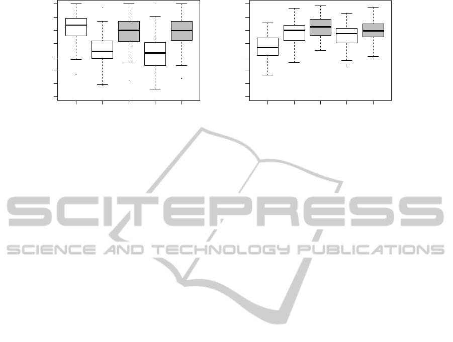
LOG B LOG+B EN LOG+EN

0.3 0.4 0.5 0.6 0.7 0.8 0.9 1.0

Methods

AUC

(a) van’t Veer.

LOG B LOG+B EN LOG+EN

0.3 0.4 0.5 0.6 0.7 0.8 0.9 1.0

Methods

AUC

(b) Pittman.

Figure 2: Breast cancer data sets. Boxplots of AUCs evaluated over 100 MCCV iterations.

MARKLAB’. The resulting data set includes 4348

genes. Clinical variables are age, tumor grade, es-

trogen receptor status, progesterone receptor status,

tumor size and angioinvasion. The second data set,

which is the Pittman data set (Pittman et al., 2004),

gives the expression levels of 12625 genes for 158

breast cancer patients. According to recurrence of

disease, 63 of these patients are classiﬁed into the

poor prognosis group, the remaining 95 patients be-

long to the good prognosis group. Gene expression

data was prepared with Affymetrix Human U95Av2

GeneChips. The data was pre-processed using pack-

ages ‘affy’ and ‘geneﬁlter’ to normalize and ﬁlter the

data. The genes that showed a low variability across

all samples were clearedout. Theresulting data set in-

cludes 8961 genes. Clinical variables are age, lymph

node status, estrogen receptor status, family history,

tumor grade and tumor size.

Figure 2 depicts AUC box plots with the breast

cancer data sets. Considering the results with the

Pittman data set, the combined models have a pos-

itive effect on prediction performances and increase

AUCs. The combined models, built with the data of

van’t Veer, do not improve AUC performances and

it is better to use for prediction of prognosis clinical

data alone. The conclusion with the van’t Veer data

set also corresponds with ﬁndings, e.g. (Gruvberger

et al., 2003).

The performances of the combined models are

similar. LOG+B seems to perform slightly better than

LOG+EN with breast cancer data sets.

Execution Times

The execution times of the combined models are

mostly based on the execution times of the models

built with high-dimensional data, therefore we com-

pared the execution times of the FGD boosting algo-

rithm from the package ‘mboost’ (B,LOG+B) with

the CCD algorithm from the package ‘glmnet’ (EN,

LOG+EN). Figure 3 depicts the comparison. Increas-

ing numbers of variables are on the horizontal axes,

while total execution times for 100 MCCV iterations

(in minutes) are on the vertical axes. The plots indi-

cate that both methods achieve similar time values.

The execution times grow linearly. Besides, FGD

boosting grows with the number of boosting iterations

(in our simulations m

max=700

). A grid of 100 λ values

is computed in each iteration of EN. The simulations

were achieved with a standard PC (Intel T72500 Core

2 Duo 2.00 GHz, 2 GB RAM) and 32-bit operating

system.

4 CONCLUSIONS

In this paper, we combine gene expression and clini-

cal data to predict disease prognosis. We used logis-

tic regression models built by different ways. GLMs

enabled combining of these models. Two suggested

approaches were evaluated with simulated (data not

shown) and publicly available breast cancer data sets.

Both approaches performed well and showed similar

performances.

The accuracy of LOG+B has already been com-

pared with other methods from literature in (

Silhav´a

and Smrˇz, 2010). It performed the same or better

than other methods from literature. LOG+EN can

be assessed analogously because of similar prediction

performance as LOG+B. The execution times of the

combined models grow linearly and the approaches

are not time consuming.

ACKNOWLEDGEMENTS

This work was supported by the Technology Agency

COMBINING GENE EXPRESSION AND CLINICAL DATA TO INCREASE PERFORMANCE OF PROGNOSTIC

BREAST CANCER MODELS

593

0 1000 2000 3000 4000

0 1 2 3 4 5

Number of genes [−]

Time [minutes]

LOG+B

(a) B and LOG+B.

0 1000 2000 3000 4000

0 1 2 3 4 5

Number of genes [−]

Time [minutes]

LOG+EN

(b) EN and LOG+EN.

Figure 3: The comparison of computation times and their dependence on increasing number of variables. The graphs are

drawn for 100 MCCV iterations.

of the Czech Republic, project TA01010931 – GenEx

– System for support of the FISH method evaluation,

and the operational programme ’Research and De-

velopment for Innovations’ in the framework of the

IT4Innovations Centre of Excellence project, reg. no.

CZ.1.05/1.1.00/02.0070.

REFERENCES

Akaike, H. (1974). A New Look at the Statistical Model

Identiﬁcation. IEEE Trans. Automat. Contr., 19 (6),

716-723.

Amaratunga, D. and Cabrera, J. (2004). Exploration and

Analysis of DNA Microarray and Protein Array Data.

John Wiley & Sons, Hoboken.

Azuaje, F. (2010). Bioinformatics and Biomarker Dis-

covery: “Omic” Data Analysis for Personalized

Medicine. John Wiley & Sons, Singapore.

B¨uhlmann, P. and Hothorn, T. (2007). Boosting Algorithms:

Regularization, Prediction and Model Fitting. Statist.

Sci., 22, 477-505.

Friedman, J., Hastie, T., H¨oﬂing, H., and Tibshirani, R.

(2007). Pathways Coordinate Optimization. Ann.

Appl. Stat., 1, 302-332.

Friedman, J. H. (2001). Greedy Function Approximation: A

Gradient Boosting Machine. Ann. Statist., 29, 1189-

1232.

Friedman, J. H., Hastie, T., and Tibshirani, R. (2010). Reg-

ularization Paths for Generalized Linear Models via

Coordinate Descent. Journal of Statistical Software,

33 (1), 1-24.

Gevaert, O., Smet, F. D., Timmerman, D., Moreau, Y.,

and Moor, B. D. (2007). Predicting the Prognosis of

Breast Cancer by Integrating Clinical and Microar-

ray Data with Bayesian Networks. Bioinformatics, 22

(14), 147-157.

Gruvberger, S. K., Ringner, M., and Eden, P. (2003). Ex-

pression Proﬁling to Predict Outcome in Breast Can-

cer: the Inﬂuence of Sample Selection. Breast Cancer

Res., 5(1), 23-26.

Li, L. (2006). Survival Prediction of Diffuse Large-B-Cell

Lymphoma Based on both Clinical and Gene Expres-

sion Information. Bioinformatics, 22(04), 466-471.

McCullagh, P. and Nelder, J. A. (1989). Generalized Linear

Models. Chapman and Hall.

Pittman, J., Huang, E., and Dressman, H. (2004). Integrated

Modeling of Clinical and Gene Expression Informa-

tion for Personalized Prediction of Disease Outcomes.

Proc.Natl.Acad.Sci., 101(22), 8431-8436.

Silhav´a, J. and Smrˇz, P. (2010). Improved Disease Outcome

Prediction Based on Microarray and Clinical Data

Combination and Pre-validation. Biomedical Engi-

neering Systems and Technologies, 36-41.

van’t Veer, L. J., Dai, H., and van de Vijver, M. J. (2002).

Gene Epression Proﬁling Predicts Clinical Outcome

of Breast Cancer. Nature, 530-536.

Zou, H. and Hastie, T. (2005). Regularization and Variable

Selection via the Elastic Net. Journal of the Royal

Statistical Society, Series B, 67, 301-320.

ICAART 2012 - International Conference on Agents and Artificial Intelligence

594