ANALYSIS OF DEFORMATION PROCESSES

USING BLOCK-MATCHING TECHNIQUES

Alvaro Rodriguez

, Carlos Fernandez-Lozano

, Jose-Antonio Seoane

, Juan R. Rabuñal

and Julian Dorado

Information and Communications Technologies, University of A Coruña, Campus Elviña sn, 15007, A Coruña, Spain

Centre of Technological Innovation in Construction and Civil Engineering, University of A Coruña,

Campus Elviña sn, 15007, A Coruña, Spain

Keywords: Computer Vision, Optical Flow, Deformation, Block-matching.

Abstract: Non rigid motion estimation is one of the main issues in computer vision. Its applications range from civil

engineering or traffic systems to medical image analysis. The challenge consists in processing a sequence of

images from of a physical body subjected to deformation processes and extracting its displacement field. In

this paper, an iterative Block-Matching technique is proposed to measure displacements in deformable

surfaces. This technique is based on successive interpolation and smoothing phases to calculate the dense

displacement field of a body. The proposed technique was experimentally validated by studying the

Yosemite sequence and it was tested in the analysis of strength test and biomedical images.

1 INTRODUCTION

The motion estimation in deformable surfaces has

been an issue of continuous major interest in several

areas ranging image diagnosis in medicine, structure

analysis in civil engineering and others.

In a general formulation of the problem, it is

necessary to estimate the motion in a scene in a time

interval Δt. By analysing two frames; I and I’

representing the states in the instants t and t+ Δt.

Optical flow techniques are a field of computer

vision born in the 80s (Horn and Schunk, 1981).

They provide a flexible approach to extract the

motion field of a scene.

A group of these techniques, the Block-Matching

techniques, calculate the displacement from a pair of

images, dividing the first one into small regions or

blocks and finding the correspondence for each block

in the second image using a search range.

Although the Block-Matching techniques are

limited due to the size and shape of the blocks, they

have been applied successfully in several fields such

as civil engineering (Raffel et al. 2000) and in

medical image analysis (Basarab et al. 2007).

Currently it is one of the most robust methods for

extracting the displacement field of a surface without

reference points such as corners or edges.

Several contributions have been made to Block-

Matching techniques. The most important are the

inclusion of pyramidal decomposition techniques to

reduce computational cost and to avoid local minima

(Amiaz et al. 2007), the use of Fourier Transforms

(FTs) and subpixel estimators (Raffel et al. 2000) to

increase accuracy.

More recently, the use iterative warping

techniques have been proposed (Basarab et al. 2007 ;

Raffel et al. 2007), some models to improve the

performance with rotational displacements have been

analysed (Ng et al. 2010) and new similarity metrics

have been proposed (Grewenig et al. 2011).

2 PROPOSED TECHNIQUE

The technique proposed follows the main principles

of any block matching technique. Dividing the image

in non overlapping regular regions called blocks and

solving the correspondence problem for each block

in the next image.

The proposed algorithm calculates the motion

vectors of the scene using an iterative represented in

Fig.1. The main steps of the algorithm are the

following.

1. The sequence of images is acquired with a digital

camera or a similar device.

327

Rodriguez A., Fernandez-Lozano C., Seoane J., Rabuñal J. and Dorado J..

ANALYSIS OF DEFORMATION PROCESSES USING BLOCK-MATCHING TECHNIQUES.

DOI: 10.5220/0003872003270332

In Proceedings of the International Conference on Computer Vision Theory and Applications (VISAPP-2012), pages 327-332

ISBN: 978-989-8565-04-4

 2012 SCITEPRESS (Science and Technology Publications, Lda.)

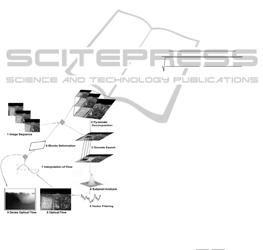
2. The image is downsampled with a standard

pyramidal decomposition algorithm.

3. A similarity metric and a search algorithm are

used to calculate the best discrete displacement.

4. The similarity values are used to perform a fitting

to a 2D Gaussian function with the Levenberg-

Marquardt technique to achieve a subpixel accuracy.

5. The obtained vectors are filtered and smoothed.

6. The optical Flow (formed by the vectors of

displacement for each block) has been obtained.

7. The Optical Flow is processed with an

interpolation algorithm, obtaining the displacements

for each pixel of each block.

8. The blocks are deformed using the information of

the displacement; a new interpolation step is required

to obtain the new blocks from the image. The new

blocks are used to improve the results from the

previous iteration or to estimate the initial position of

the blocks in the next frame.

9. If the last iteration has been performed, The

Dense Deformation Field (the vectors of

displacement for each pixel of the image) has been

obtained.

Figure 1: General scheme of the proposed algorithm.

2.1 Discrete Displacement

To measure the degree of correspondence for each

block of I with another block from I’, the proposed

algorithm uses the statistical similarity of the grey

levels in both regions.

The original block is centered in the point (i, j) in

the image I. After applying a displacement

d(i,j)=(x,y), this block will correspond with the

region centered in (i’,j’) in I’. This is described in (1).

(i', j') = (i + x, j + y) (1)

This approach is based on the assumption

expressed in (2).

I(i, j) + NF = I' (i + x, j + y) (2)

NF being a noise factor following a specific and

unknown statistical distribution, I the original image

and I' the deformed one.

To find the point (i’, j’) a set of candidate blocks

will be defined in I’ using a search range from (i, j).

Therefore, the objective will be to find the candidate

region maximizing a similarity function with the

original one.

In this work, the Pearson's correlation quotient

(R) is used to that end (3).

()

(

)

(

)

(

)

()

´´

,,´'

(', ')

,´´,´'

Iij I i j

Rij

Iij I i j

μμ

−× −

−−

∑

∑∑

(3)

Where N is the size of the block, µ and µ’ are the

average intensity values of the blocks centered in

I(i,j) and I'(i',j') respectively.

The chosen metric (R) has the advantages of

being invariant to the average gray level and

therefore it is robust in presence of some natural

variability processes such as those present in

common light sources.

2.2 Subpixel Accuracy

The accuracy of the technique presented so far is

limited to the pixel level due to the digital nature of

the images.

However, the correlation value itself contains

some useful information, given that the values

achieved in the pixels surrounding the best value will

reflect one part of the displacement located between

both pixels.

Thus, the correlation can be translated to a

continuous space using a numerical fitting technique.

Here, the two-dimensional Gaussian function defined

in (4) has been used as a continuous model of the

correlation values.

()()

(, )

fxy e

μμ

σσ

⎡

⎤

−−

⎢

⎥

−+

⎢

⎥

××

⎣

⎦

=×

(4)

Being λ, µ

and σ

the parameters of the

function. This parameters are calculated by

performing a fitting using the Levenberg-Marquardt

(LM) method as defined in (5).

VISAPP 2012 - International Conference on Computer Vision Theory and Applications

328

(

)

() ()

55 55151

...

λλ

... ... ...

...

nn n n

JdIIncJ E

fxy fxy

σσ

×× ×××

×+×× = ×

⎡⎤

∂∂

⎢⎥

∂∂

⎢⎥

∂∂

⎢⎥

∂∂

⎣⎦

(5)

With d

∈

, d ≠ 0 adjusted for each algorithm

iteration, E is the error matrix, J the Jacobian matrix

of f and Inc the vector of increments for the next

iteration.

The following initial estimation for the function

parameters have been used: λ=max(R

), µx= 0,

µy=0, σx=2 and σy= 2.

The algorithm for updating d is shown in (6).

According to it, the Residual Sum of Squares (RSS)

is calculated from the error matrix (E), so that if the

RSS decreases, the d value is fixed to a constant near

to 0, so the algorithm gets close to the Gauss-Newton

one; in other instances, the d value increases so that

the algorithm behaves as a gradient descent method.

()

110

kkk

kkkk

k kMax d dMax FINISH

RSS RSS d d v

RSS RSS d d v v v

−+

=−

⎧

−≥ > ⇒

⎪

<=−=

⎨

⎪

≥=×=×

⎪

⇒

⎩

⇒

∪

(6)

Where kMax and dMax can be adjusted by the user.

2.3 Vector Filtering

Once the displacement vectors have been calculated,

a vector processing algorithm has been used to

replace the anomalous vectors and to obtain a soft

vector field. This is done in two steps:

1. First, the root mean square (RMS) of the

neighbors of each vector is calculated. If the

difference of this value with the estimated one is

greater than a threshold set by the user, the vector is

replaced by the RMS.

2. Finally, the vector field is smoothed with a

bidimensional Gaussian filter. The default filter uses

a 3x3 sized window.

2.4 Deformation of the Blocks

It should be noted that, if non-rigid displacements are

considered the assumption expressed in (2) is

generally false because neither rotation nor second

order effects are included in the model.

Generally, it can be assumed that if the regions or

blocks are small enough, then the second order

effects may be disregarded and strains can be

calculated from the locally linear displacements in

every region.

If deformations are considered, the objects in the

scene start in an initial non-deformed stage and

develop to a final deformed one. The same principle

can be applied to blocks. They start with a regular

rectangular shape and, using the information from the

measured displacement, the shape of the block can be

changed according to the deformations of the body in

the scene.

Thus, using the vector field obtained in the

previous iteration or from a previous frame of the

scene, a dense displacement field is obtained by

interpolating the motion vectors.

The dense field can be used to obtain the new

positions of the pixels in the block and with this

information a second interpolation step can be used

to obtain the deformed block.

The deformed block is used to improve the

measurement from the previous iteration or to predict

the shape of the surface in the next frame.

In the presented work, bilinear and bicubic B-

spline interpolation methods were used to interpolate

the displacement field and the data of the block

respectively.

3 EXPERIMENTAL RESULTS

3.1 Synthetic Images

The first assay was performed with synthetic images.

In this experiment, the Yosemite synthetic sequence

was used. This is a standard test for benchmarking

optical flow algorithms. It was created by Lynn

Quam (Heeger, 1987) and it was widely studied in

different works (Austvoll, 2005).

Besides, this sequence is one of the best to

perform a evaluation of a Block-Matching algorithm,

since it contains a single surface with a complex

motion, which is the kind of motion where the use

Block-Matching technique makes sense.

This experiment was performed analyzing the

motion between consecutive frames, calculating the

statistics of error according to the true ground data

and using the metrics and methodologies published

in (Scharstein et al. 2007). According to this, the

error was calculated using the dense displacement

field except a border region with a size of 10 pixels

(7).

The obtained results were calculated using non

overlapped blocks of 15x15 pixels and 5 iterations.

An example of obtained results is shown in Fig.2.

ANALYSIS OF DEFORMATION PROCESSES USING BLOCK-MATCHING TECHNIQUES

329

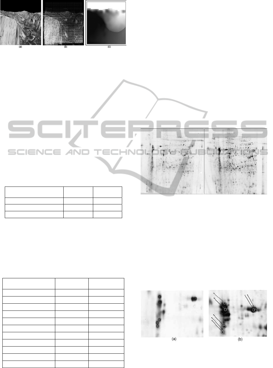
Figure 2: Yosemite experiment. (a) First frame (b) Last

frame and motion vectors of the blocks. (c) Dense motion

field (gray level represents the magnitude of the

displacement).

Table 1 shows the comparative results with other

block matching methods. The following techniques

were used:

1. The DaVis system, from LA Vision (PIV, 2011).

It is a block-matching based technique introduced in

(Raffel et al. 2000) and enhanced in (Raffel et al.

2007). It has been widely used in publications and

experiments in various fields (Deng et al. 2004).

2. The Block-Matching technique provided by the

computer vision library OpenCv available at

(

OPENCV, 2011).

Table 1: Comparative results in the Yosemite sequence

using Block-Matching algorithms.

Algorithm

Average

Error

SSD Error

This Work

0.11

LaVision (Raffel et al. 2007) 0.26

0.26

OpenCv (OPENCV, 2011)

0.43

0.55

Table 2 shows the results obtained with the

proposed technique compared with those obtained by

the top 15 grayscale algorithms from the Middlebury

Ranking.

Table 2: Comparative results in the Yosemite sequence

using the top 10 grayscale algorithms of the Middlebury

ranking. More results and references are available in [4]

Algorithm

Average

Error

SSD Error

2D-CLG 0.10 0.10

This Work

0.11

GroupFlow 0.11 0.26

LocallyOriented 0.12 0.11

Ad-TV-NDC 0.12 0.14

Modified CLG 0.12 0.16

Dynamic MRF 0.13 0.14

F-TV-L1 0.13 0.14

Learning Flow 0.14 0.16

Adaptive 0.14 0.17

Nguyen 0.14 0.13

The proposed technique obtained much better

results than the tested block matching technique and

the second best results for grayscale optical flow

algorithms in the Middlebury ranking.

3.2 Application Field: 2D Gel Images

In proteomics, to separate proteins obtained from a

sample the two-dimensional electrophoresis is

commonly used. After the proteins have been

separated, each dark spot represents different kind of

proteins present in the sample and its size depends on

the amount of protein.

In a typical association study, images are

compared in pairs to find differences in proteins of

interest. For this purpose, it is necessary to find the

spot correspondence in the images (Almansa et al.

2007).

Figure 3: Example of two images in a 2D Gel experiment

where it is necessary to find a spot correspondence.

The task is nowadays a bottleneck in the

proteomics research (Voss and Haberl, 2000) and

automatic analysis techniques can improve this

process considerably.

The proposed technique has been used to match

proteins of interest in 2D gel images. With this

purpose blocks were defined using the position of the

proteins in a reference frame and a simple analysis

was performed avoiding the filtering and smoothing

steps. This procedure is shown in Fig.4.

Figure 4: 2D Gel experiment. (a) Reference frame with

marked proteins. (b) Protein displacement to achieve its

final position in test image.

VISAPP 2012 - International Conference on Computer Vision Theory and Applications

330

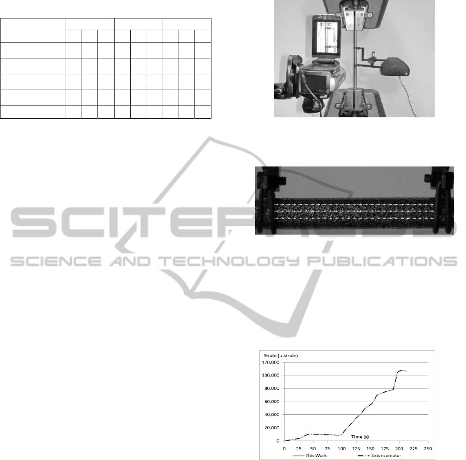
Table 3: Comparative results in proteomics.

Algorithm

Easy Medium Complex

cor

inc

% n

cor

inc

% n

cor

inc

This Work 204 4 98.1 154 4 97.5 46 9 83.7

Hybrid (Wrz et al. 2008)

203 5 97.6 153 5 96.8 - - -

Intensity (Wrz et al. 2008)

200 8 96.2 150 8 94.9 - - -

Hybrid (Rohr et al. 2004)

201 7 96.6 149 9 94.3 - - -

Intensity (Rohr et al. 2004)

187 21 89.9 137 21 86.7 - - -

The data used in the present work was built using

images extracted from the Wolfson MIC Laboratory

test sequences. In these data, every couple of images

was assigned a complexity level according to the

criterion of an expert.

Obtained results are shown in and summarized in

Table 3. These results were compared with those

published in (Rohr, 2004) and (Wrz et al. 2008)

where the same data is used (although no results with

high complexity images are provided).

Analysing the obtained results, it may be seen

that the success rates obtained with biomedical

images were higher than the rates reached by specific

works using the same data.

3.3 Application Field: Strength Tests

Some of the main needs in Civil Engineering are to

know the stress-strain response of materials used

structures. For this purpose, strength tests are usually

carried out by applying controlled loads or strains to

a test model.

In, strength tests, information about the material's

behavior is traditionally obtained using strain gauges

or extensometers, these devices are expensive or non

reusable and they must be physically linked to the

material interfering with the experiment. Furthermore

these devices provide only information about the

length variation of the structure in a given point and

in a single direction.

The proposed technique can be used to extract the

full displacement field of the body without

considering the points of interest or the main

direction of deformation in the body.

In the next assay, a tensile test was performed

with a cylindrical aluminum bar of 30cm length x

8mm diameter. The experiment was recorded with a

video camera and the calibration technique proposed

in (Zhang, 1999) was used to obtain measurements in

a real scale. Fig.5 and Fig.6 illustrate how

measurements were performed.

A traditional contact extensometer was used in

this assay to compare the obtained results with those

provided by traditional instrumentation.

Figure 5: 2D Gel experiment. (a) Reference frame with

marked proteins. (b) Protein displacement to achieve its

final position in test image.

Figure 6: Displacement vectors estimated during the test

and the extensometer attached to the material.

The vertical strain obtained (expressed in µ

strains) for the section of the aluminum bar where the

extensometer has been attached is shown in Fig.7.

Analysing the obtained results it may be seen that

the proposed technique produces virtually identical

results to those by extensometer.

Figure 7: Graphic of the test with the aluminum. Strain

obtained with the extensometer is shown together with the

strain measured with the proposed technique.

4 CONCLUSIONS

The present paper introduces a new technique to

analyze general deformable displacements in

different surfaces without using displacement or

deformation models.

The obtained results show that the proposed

technique can retrieve the complete displacement

field of a surface, obtaining accurate and robust

results.

ANALYSIS OF DEFORMATION PROCESSES USING BLOCK-MATCHING TECHNIQUES

331

In the analysis of 2D gel images better results

than specific works in the field were obtained and in

the analysis of strength test the same precision as

traditional devices was obtained avoiding the

limitations of contact sensors.

ACKNOWLEDGEMENTS

This work was partially supported by the General

Directorate of Research, Development and Innovation of

the Xunta de Galicia (Ref. 08TMT005CT), grant

(Ref.10SIN105004PR) funded by Xunta de Galicia and

Consellería of Economy and Industry of the Xunta de

Galicia (Ref. 10MDS014CT).

REFERENCES

Almansa A, Gerschuni M, Pardo A and Preciozzi J: 2007.

Processing of 2D Electrophoresis Gels Iccv -

Workshop on Computer Vision Applications for

Developing Countries.

Amiaz T, Lubetzky E and Kiryati N: 2007. Coarse to

overfine optical flow estimation.Pattern Recognition.

40(9):2494-1503.

Austvoll I: 2005. A study of the yosemite sequence used as

a test sequence for estimation of optical flow. Lecture

Notes in Computer Science. 3540(2005):659-668.

Baker S, Scharstein D and Lewis JP. Middlebury

computer vision pages, an evaluation of optical flow

algorithms. http://vision.middlebury.edu/ow/eval.

(Accessed: 2011).

Basarab. A, Aoudi W, Liebgott H, Vray D and Delachartre

P. Parametric Deformable Block Matching for

Ultrasound Imaging. IEEE International conference

on Image Processing. (2007).

Deng Z, Richmond MC, Guest GR and Mueller RP: 2004.

Study of Fish Response Using Particle Image

Velocimetry and High-Speed, High-Resolution

Imaging, Technical Report PNNL-14819.

Grewenig S, Zimmer S and Weickert J: 2011. Rotationally

invariant similarity measures for nonlocal image

denoising. Journal of Visual Communication and

Image Representation. 22(2):117-130.

Heeger D: 1987. Model for the extraction of image flow.

Journal of the Optical Society of America A: Optics,

Image Science, and Vision 4(1987):1455–1471.

Horn BKP and Schunk BG: 1981. Determining optical

flow. Artificial Intelligence 17:185-203.

Ng KH, Po LM, Cheung KW and Wong KM: 2010.

Block-Matching Translational and Rotational Motion

Compensated Prediction Using Interpolated Reference

Frame. Journal on Advances in Signal Processing.

OPENCV. Open Source Computer Vision.

http://opencv.willowgarage.com (Accessed: 2011).

PIV. Particle image Velocimetry. http://www.piv.de

(Accessed: 2011).

Raffel M, Willert C and Kompenhans J: 2000. Particle

image velocimetry, a practical guide. Springer, Berlin.

Raffel M, Willert C and Kompenhans J: 2007. Particle

image velocimetry, a practical guide, Second Edition.

Springer, Berlin.

Rohr K, Cathier P and Wrz S: 2004. Elastic registration of

electrophoresis images using intensity information and

point landmarks. Pattern Recognition 37:035-1048 .

Scharstein D, Baker S, and Lewis JP: 2007. A database

and evaluation methodology for Optical Flow. ICCV.

Voss T and Haberl P: 2000. Observations on the

reproducibility and matching effciency of two-

dimensional electrophoresis gels: consequences for

comprehensive data analysis. Electrophoresis

21:3345-3350.

Wrz S, Winz M and Rohr K: 2008. Geometric alignment

of 2D gel electrophoresis images using physics-based

elastic registration. IEEE International Symposium on

Biomedical Imaging: From Nano to Macro.

Zhang: 1999. Flexible Camera Calibration by Viewing a

Plane From Unknown Orientations. IEEE International

Conference on Computer Vision. 1: 666-673.

VISAPP 2012 - International Conference on Computer Vision Theory and Applications

332