DETECTOR OF FACIAL LANDMARKS LEARNED

BY THE STRUCTURED OUTPUT SVM

Michal U

r, Vojt

ech Franc and V

aclav Hlav

Center for Machine Perception, Department of Cybernetics, Faculty of Electrical Engineering,

Czech Technical University in Prague, Technick

a 2, 166 27 Prague 6, Czech Republic

Keywords:

Facial Landmark Detection, Structured Output Classiﬁcation, Support Vector Machines, Deformable Part

Models.

Abstract:

In this paper we describe a detector of facial landmarks based on the Deformable Part Models. We treat the task

of landmark detection as an instance of the structured output classiﬁcation problem. We propose to learn the

parameters of the detector from data by the Structured Output Support Vector Machines algorithm. In contrast

to the previous works, the objective function of the learning algorithm is directly related to the performance of

the resulting detector which is controlled by a user-deﬁned loss function. The resulting detector is real-time on

a standard PC, simple to implement and it can be easily modiﬁed for detection of a different set of landmarks.

We evaluate performance of the proposed landmark detector on a challenging “Labeled Faces in the Wild”

(LFW) database. The empirical results demonstrate that the proposed detector is consistently more accurate

than two public domain implementations based on the Active Appearance Models and the Deformable Part

Models. We provide an open-source implementation of the proposed detector and the manual annotation of

the facial landmarks for all images in the LFW database.

1 INTRODUCTION

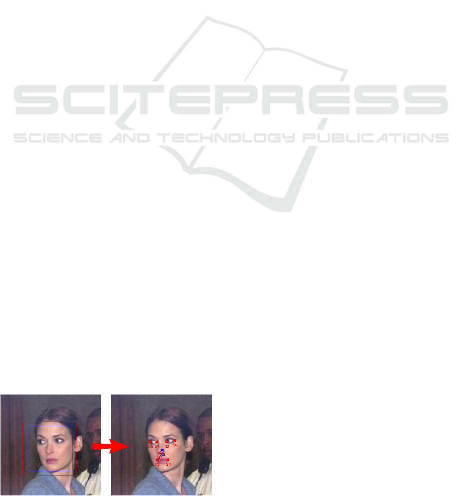
The detection of facial landmarks like canthi, nose

and mouth corners (see Figure 1) is an essential part

of face recognition systems. The accuracy of the de-

tection signiﬁcantly inﬂuences its ﬁnal performance

(Beumer and Veldhuis, 2005; Cristinacce et al., 2004;

Riopka and Boult, 2003). The problem of the precise

and robust detection of facial landmarks has received

a lot of attention in the past decade. We brieﬂy review

only the approaches relevant to the method proposed

in this paper.

Among the most popular are detectors based on

the Active Appearance Models (AAM) (Cootes et al.,

Figure 1: Functionality of the facial landmark detector.

2001) which use a joint statistical model of appear-

ance and shape. Detectors build on AAM provide a

dense set of facial features, allowing to extract whole

contours of facial parts like eyes, etc. However high

resolution images are required for both training and

testing stage and the detection leads to solving a non-

convex optimization problem susceptible to local op-

tima unless a good initial guess of the landmark posi-

tions is available.

A straightforward approach to landmark detec-

tion is based on using independently trained detectors

for each facial landmark. For instance the AdaBoost

based detectors and its modiﬁcations have been fre-

quently used (Viola and Jones, 2004). If applied in-

dependently, the individual detectors often fail to pro-

vide a robust estimate of the landmark positions. The

weakness of the local evidence can be compensated

by using a prior on the geometrical conﬁguration of

landmarks. The detection is typically carried out in

two consecutive steps. In the ﬁrst step, the individ-

ual detectors are used to ﬁnd a set of candidate po-

sitions for each landmark separately. In the second

step, the best landmark conﬁguration with the highest

support from the geometrical prior is selected. The

landmark detectors based on this approach were pro-

547

r M., Franc V. and Hlavá

c V..

DETECTOR OF FACIAL LANDMARKS LEARNED BY THE STRUCTURED OUTPUT SVM.

DOI: 10.5220/0003863705470556

In Proceedings of the International Conference on Computer Vision Theory and Applications (VISAPP-2012), pages 547-556

ISBN: 978-989-8565-03-7

 2012 SCITEPRESS (Science and Technology Publications, Lda.)

posed for example in (Beumer et al., 2006; Cristi-

nacce and Cootes, 2003; Erukhimov and Lee, 2008;

Wu and Trivedi, 2005).

The Deformable Part Models (DPM) (Crandall

et al., 2005; Felzenszwalb and Huttenlocher, 2005;

Felzenszwalb et al., 2009; Fischler and Elschlager,

1973) go one step further by fusing the local appear-

ance model and the geometrical constraints into a sin-

gle model. The DPM is given by a set of parts along

with a set of connections between certain pairs of

parts arranged in a deformable conﬁguration. A nat-

ural way how to describe the DPM is an undirected

graph with vertices corresponding to the parts and

edges representing the connections between the pairs

of connected parts. The DPM detector estimates all

landmark positions simultaneously by optimizing a

single scoring function composed of a local appear-

ance model and a deformation cost. The complexity

of ﬁnding the best landmark conﬁguration depends on

the structure of underlying graph. Acyclic graph al-

lows efﬁcient estimation by a variant of the Dynamic

Programming (DP).

An instance of ﬁnely tuned facial landmark detec-

tor based on the DPM has been proposed in (Ever-

ingham et al., 2006). The very same detector was

also used in several successful face recognition sys-

tems described in (Everingham et al., 2009) and (Sivic

et al., 2009). In this case, the local appearance model

is learned by a multiple-instance variant of the Ad-

aBoost algorithm with Haar-like features used as the

weak classiﬁers. The deformation cost is expressed

as a mixture of Gaussian trees whose parameters are

learned from examples. This landmark detector is

publicly available and we use it for comparison with

our detector

. Importantly, learning of the local ap-

pearance model and the deformation cost is done in

two independent steps which simpliﬁes learning, but

may not be optimal in terms of detectors accuracy.

We propose to learn the parameters of the DPM

discriminatively in one step by directly optimizing ac-

curacy of the resulting detector. The main contribu-

tions of this paper are as follows:

1. We treat the landmark detection with the DPM as

an instance of the structured output classiﬁcation

problem whose detection accuracy is measured by

a loss function natural for this application. We

propose to use the Structured Output SVM (SO-

SVM) (Tsochantaridis et al., 2005) for supervised

learning of the parameters of the landmark detec-

tor from examples. The learning objective of the

There also exists a successful commercial so-

lution OKAO Vision Facial Feature Extraction API

(http://www.omron.com) which is used for example in

Picasa

or Apple iPhoto

software.

SO-SVMs is directly related to the accuracy of the

detector. In contrast, all existing approaches we

are aware of optimize surrogate objective func-

tions whose relation to the detector accuracy is not

always clear.

2. We empirically evaluate accuracy of the proposed

landmark detector learned by the SO-SVMs on a

challenging “Labeled Faces in the Wild” database

(Huang et al., 2007).

3. We provide an empirical comparison of two popu-

lar optimization algorithms — the Bundle Method

for Regularized Risk Minimization (BMRM) (Teo

et al., 2010) and the Stochastic Gradient Descend

(SGD) (Bordes et al., 2009) — which are suit-

able for solving the convex optimization problem

emerging in the SO-SVM learning.

4. We provide an open source library which imple-

ments the proposed detector and the algorithm for

supervised learning of its parameters. In adidtion

we provide a manual annotation of the facial land-

marks for all images from the LFW database.

The paper is organized as follows. Section 2 de-

ﬁnes the structured output classiﬁer for facial land-

mark detection based on the DPM. Section 3 de-

scribes the SO-SVM algorithm for learning the pa-

rameters of the classiﬁer from examples. Experimen-

tal results are presented in Section 4. Section 5 shortly

describes the open source implementation of our de-

tector and the provided manual annotation of the LFW

database. Section 6 concludes the paper.

2 THE STRUCTURED OUTPUT

CLASSIFIER FOR FACIAL

LANDMARK DETECTION

We treat the landmark detection as an instance of

the structured output classiﬁcation problem. We as-

sume that the input of our classiﬁer is a still image

of ﬁxed size containing a single face. In our exper-

iments we construct the input image by cropping a

window around a bounding box found by a face de-

tector (enlarged by a ﬁxed margin ensuring the whole

face is contained) and normalizing its size. The clas-

siﬁer output are estimated locations of a set of facial

landmarks. A formal deﬁnition is given next.

Let J = X

H×W

be a set of input images with

H × W pixels where X denotes a set of pixel val-

ues which in our experiments, dealing with 8bit gray-

scale images, is X = {0, ..., 255}. We describe the

conﬁguration of M landmarks by a graph G = (V,E),

where V = {0,. .. ,M − 1} is a set of landmarks and

VISAPP 2012 - International Conference on Computer Vision Theory and Applications

548

face center

canthus-rl

canthus-lr

mouth-corner-r

canthus-rr

canthus-ll

nose

(a) (b)

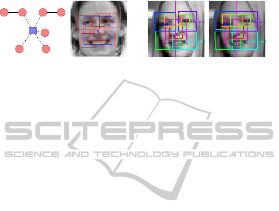
Figure 2: Deﬁnition of (a) the underlying graph G = (V,E)

for the landmark conﬁguration and (b) the components of

the proposed detector.

E ⊂ V

is a set of edges deﬁning the neighbouring

landmarks. Each landmark is assigned a position s

∈

⊂ {1,...,H} × {1,. .. ,W } where S

denotes a set

of all admissible positions of the i-th landmark within

the image I ∈ J . The quality of a landmark conﬁgura-

tion s = (s

,. .. ,s

M−1

) ∈ S = S

×···×S

M−1

given an

input image I ∈ J is measured by a scoring function

f : J × S → R deﬁned as

f (I,s) =

∑

i∈V

(I,s

) +

∑

(i, j)∈E

i j

) . (1)

The ﬁrst term in (1) corresponds to a local appear-

ance model evaluating the match between landmarks

on positions s and the input image I. The second term

in (1) is the deformation cost evaluating the relative

positions of the neighboring landmarks i and j.

We assume that the costs q

: J × S

→ R,i =

0,. .. ,M − 1 and g

i j

: S

× S

→ R,(i, j) ∈ E are lin-

early parametrized functions

(I,s

) = hw

,Ψ

(I,s

)i (2)

i j

) = hw

i j

,Ψ

i j

)i, (3)

where Ψ

: J × S

→ R

, Ψ

i j

: S

× S

→ R

,i =

0,. .. ,M −1 are predeﬁned maps and w

∈ R

i j

∈

,i = 0, .. ., M −1 are parameter vectors which will

be learned from examples. Let us introduce a joint

map Ψ : J × S → R

and a joint parameter vector

w ∈ R

deﬁned as a column-wise concatenation of

the individual maps Ψ

,Ψ

i j

and the individual param-

eter vectors w

i j

respectively. With these deﬁni-

tions we see that the scoring function (1) simpliﬁes to

f (I,s) =

w,Ψ(I, s)

Given an input image I, the structured output clas-

siﬁer returns the conﬁgurations

s computed by maxi-

mizing the scoring function f (I,s), i.e.

s ∈ argmax

s∈S

f (I,s) . (4)

We assume that the graph G = (V,E) is acyclic (see

Figure 2(a)), which allows efﬁcient solving of the

maximization problem (4) by dynamic programming.

Figure 3: Left: optimal search spaces for each component.

Right: the same search spaces made symmetrical along the

vertical magenta line.

A complete speciﬁcation of the structured classi-

ﬁer (4) requires to deﬁne:

• The maps Ψ

(I,s

),i = 0,...,M − 1 where

(I,s

) deﬁnes a local feature descriptor of i-th

landmark computed on a rectangular window cen-

tered at s

. We call the rectangular window a com-

ponent (see Figure 2(b)). The size of the compo-

nent and its feature descriptor are crucial design

options which have to be made carefully. In Sec-

tion 2.1 we describe a list of feature descriptors

we have considered.

• The ﬁxed maps Ψ

i j

),(i, j) ∈ E deﬁning the

parametrization of the deformation cost. Section

2.2 describes the parametrization which we have

considered.

• The set S = (S

× ··· × S

M−1

) deﬁning the search

space of the landmark positions. These sets can

be interpreted as hard constraints on the admissi-

ble conﬁgurations of the landmarks, i.e. the land-

mark positions outside these sets corresponds to

−∞ value of the deformation cost g

i j

We tune the size of these search spaces ex-

perimentally — we keep track of the axis

aligned bounding box (AABB) for each compo-

nent trough the whole database excluding the im-

ages whose components does not ﬁt in the image.

We set the size of components in order to keep at

least 95% images of the original database. Con-

sequently, the AABB of each component is made

vertically symmetric along the center y-axis in or-

der to remove bias to certain positions. Figure 3

visualizes the found search spaces.

• The joint parameter vector w ∈ R

learned from

the training examples by the SO-SVM algorithm

described in Section 3.

Finally we would like to stress that the particular

number of landmarks and their neighborhood struc-

ture can be arbitrary as long as the inference prob-

lem (1) can be solved efﬁciently. In this paper we

experiment with the 8-landmarks variant of the graph

DETECTOR OF FACIAL LANDMARKS LEARNED BY THE STRUCTURED OUTPUT SVM

549

G = (V,E) shown in Figure 2(a).

2.1 Appearance Model

We have experimented with several feature descrip-

tors Ψ

for the local appearance model q

(I,s

). In

particular, we considered i) normalized intensity val-

ues, ii) derivatives of image intensity values, iii) his-

tograms of Local Binary Patterns (LBP) (Heikkil

et al., 2009) and iv) the LBP pyramid feature descrip-

tor (Franc and Sonnenburg, 2010). We obtained the

best results with the LBP pyramid feature descriptor

which is used in the experiments. The LBP pyramid

descriptor is constructed by concatenating binary en-

coded LBP features computed in each pixel (up to

boundary pixels) and in several scales. In particular,

we use the LBP pyramid computed in 4 scales starting

from the original image and consequently downscal-

ing the image 3 times by 1/2. The resulting feature

vector is high dimensional but very sparse.

2.2 Deformation Cost

We have experimented with two parametrizations of

the deformation cost g

i j

): i) a table represen-

tation and ii) a quadratic function of a displacement

vector between landmark positions.

The table representation is the most generic form

of the deformation cost useful when no prior knowl-

edge is available. Table elements specify cost for each

combination of s

and s

separately. Ψ

i j

) is a

sparse vector with all elements zero but the element

corresponding to the combinations (s

) which is

one. Though the table representation is very ﬂexi-

ble its main disadvantage is a very large number of

parameters to be learned. In turn, a large number of

training examples is required to avoid over-ﬁtting.

As the second option, we considered the defor-

mation cost g

i j

) to be a quadratic function of a

displacement vector s

− s

. Following (Felzenszwalb

et al., 2009), we deﬁne the deformation cost as

i j

) = (dx,dy, dx

,dy

)

(dx,dy) = (x

) − (x

)



(5)

This representation accounts for the distance and the

direction of the j-th landmark with respect to i-th

landmark. This representation is determined only by

four parameters which substantially reduces the risk

of over-ﬁtting.

We found experimentally the quadratic deforma-

tion cost to give slightly better results compared to

the table representation.

3 LEARNING THE PARAMETERS

OF THE STRUCTURED

OUTPUT CLASSIFIER

We learn the joint parameter vector w by the SO-SVM

algorithm (Tsochantaridis et al., 2005). The require-

ments on the classiﬁer are speciﬁed by a user deﬁned

loss-function L : S × S → R. The value L(s,s

∗

) pe-

nalizes the classiﬁer estimate s provided the actual

conﬁguration of the landmarks is s

∗

. The SO-SVM

requires loss function to be non-negative and zero iff

the estimate is absolutely correct, i.e. L(s,s

∗

) ≥ 0,

∀s,s

∗

∈ S , and L(s,s

∗

) = 0 iff s = s

∗

. In particular,

we use the mean normalized deviation between the

estimated and the ground truth positions as the loss

function, i.e.,

L(s,s

∗

) = κ(s

∗

)

M−1

∑

j=0

− s

∗

k. (6)

The normalization factor κ(s

∗

) = k

eyeR

+ s

eyeL

) −

mouth

−1

is reciprocal to the face size which we

deﬁne as the length of the line connecting the mid-

point between the eye centers s

eyeR

and s

eyeL

with the

mouth center s

mouth

. The normalization factor is in-

troduced in order to make the loss function scale in-

variant which is necessary because responses of the

face detector used to construct the input images do

not allow accurate estimation of the scale. Figure 4

illustrates the meaning of the loss function (6). Fi-

nally, we point out that any other loss function meet-

ing the constraints deﬁned above can be readily used,

e.g. one can use maximal normalized deviation.

Given a set of training examples

{(I

),. .. ,(I

)} ∈ (J × S )

composed of

pairs of the images and their manual annotations,

the parameter w of the classiﬁer (4) is obtained by

solving the following convex minimization problem

∗

= argmin

w∈R



kwk

+ R(w)



, where (7)

R(w) =

∑

i=1

max

s∈S



L(s

,s) +



w,Ψ(I

,s)





−

∑

i=1



w,Ψ(I

)



(8)

The number λ ∈ R

is a regularization constant

whose optimal value is tuned on a validation set. R(w)

is a convex piece-wise linear upper bound on the em-

pirical risk

∑

i=1

L(s

,arg max

s∈S

f (I

,s)). That is,

the learning algorithm directly minimizes the perfor-

mance of the detector assessed on the training set and

at the same time it controls the risk of over-ﬁtting via

the norm of the parameter vector.

VISAPP 2012 - International Conference on Computer Vision Theory and Applications

550

Though the problem (7) is convex its solving is

hard. The hardness of the problem can be seen when it

is expressed as an equivalent quadratic program with

m|S | linear constrains (recall that |S | is the number

of all landmark conﬁgurations). This fact rules out

off-the-shelf optimization algorithms.

Thanks to its importance a considerable effort has

been put to a development of efﬁcient optimization

algorithms for solving the task (7). There has been

an ongoing discussion in the machine learning com-

munity trying to decide whether approximative on-

line solvers like the SGD are better than the accurate

slower solvers like the BMRM. No deﬁnitive consen-

sus has been achieved so far. We contribute to this

discussion by providing an empirical evaluation of

both approaches on the practical large-scale problem

required to learn the landmark detector. The empir-

ical results are provided in section 4.5. For the sake

of self-consistency, we brieﬂy describe the considered

solvers, i.e. the BMRM and the SGD algorithm, in the

following two sections.

3.1 Bundle Methods for Regularized

Risk Minimization

The BMRM is a generic method for minimization of

regularized convex functions (Teo et al., 2010), i.e.

BMRM solves the following convex problem

∗

= argmin

w∈R

F(w) :=

kwk

+ R(w),

where R : R

→ R is an arbitrary convex function.

The risk term R(w) is usually the complex part of the

objective function which makes the optimization task

hard. The core idea is to replace the original problem

by its reduced problem

= argmin

w∈R

(w) :=

kwk

+ R

(w) . (9)

The objective function F

(w) of the reduced prob-

lem (9) is obtained after replacing the risk R(w) in

the original objective F(w) by its cutting plane model

(w) = max

i=0,1,...,t−1



R(w

+ hR

),w −w



, (10)

where R

) ∈ R

denotes a subgradient of R(w)

evaluated at the point w

∈ R

Starting from an initial guess w

= 0, the BMRM

algorithm computes a new iterate w

by solving the

reduced problem (9). In each iteration t, the cutting

plane model (10) is updated by a new cutting plane

computed at the intermediate solution w

leading to

a progressively tighter approximation of F(w). The

BMRM algorithm halts if the gap between F(w

) (an

upper bound on F(w

∗

)) and F

) (a lower bound on

F(w

∗

)) falls below a desired ε, meaning that F(w

) ≤

F(w

∗

) + ε. The BMRM algorithm halts after at most

O(1/ε) iterations for arbitrary ε > 0 (Teo et al., 2010).

The reduced problem (9) can be expressed as an

equivalent convex quadratic program with t variables.

Because t is usually small (up to a few hundreds), off-

the-shelf QP solvers can be used.

Before applied to a particular problem, the

BMRM algorithm requires a procedure which for a

given w returns the value of the risk R(w) and its sub-

gradient R

(w). In our case the risk R(w) is deﬁned

by (8) and its sub-gradient can be computed by the

Danskin’s theorem as

(w) =

∑

i=1



Ψ(I

) − Ψ(I

)



, (11)

= argmax

s∈S

L(s

,s) +



w,Ψ(I

,s)



.(12)

Note that the evaluation of R(w) and R

(w) is dom-

inated by the computation of the scalar products

hw,Ψ(I

,s)i, i = 1, .. ., m, s ∈ S , which, fortunately,

can be efﬁciently parallelized.

3.2 Stochastic Gradient Descent

Another popular method solving (7) is the Stochastic

Gradient Descent (SGD) algorithm. We use the mod-

iﬁcation proposed in (Bordes et al., 2009) which uses

two neat tricks. Starting from an initial guess w

, the

SGD algorithm iteratively changes w by applying the

following rule:

t+1

= w

−

−1

, g

= λw

+ h

(13)

is a constant and t is the number of the iteration.

The SGD implementation proposed in (Bordes et al.,

2009) tunes the optimal value of t

on a small por-

tion of training examples sub-sampled from training

set. The sub-gradient is computed in almost the same

manner as in (11), but only for one training image at

a time, i.e., h

= Ψ(I

) − Ψ(I

In addition, (Bordes et al., 2009) propose to ex-

ploit the sparsity of the data in the update step. The

equation (13) can be expressed as

t+1

= w

− α

− β

, where (14)

α =

, β =

−1

(15)

Note that if h

is sparse then subtracting β

in-

volves only the nonzero coefﬁcients of h

, but sub-

tracting α

involves all coefﬁcients of w

. In turn, it

is beneﬁcial to reformulate the equation (14) as

t+1

= (1 − α

− β

. (16)

DETECTOR OF FACIAL LANDMARKS LEARNED BY THE STRUCTURED OUTPUT SVM

551

By using this trick, the complexity O(d) corre-

sponding to the na

ıve implementation of the update

rule (13) reduces to the complexity O(d

non−zero

) cor-

responding to the reformulated rule (16), where d is

the dimension of the parameter vector and d

non−zero

the number of the non-zero elements in h

. Typically,

like in our case, d

non−zero

is much smaller than d.

A considerable advantage of the SGD algorithm

is its simplicity. A disadvantage is that the SGD al-

gorithm does not provide any certiﬁcate of optimality

and thus theoretically grounded stopping condition is

not available.

4 EXPERIMENTS

In this section, we present experimental evaluation of

the proposed facial landmark detector and its com-

parison against three different approaches. We con-

sidered the detector estimating positions of the eight

landmarks: the canthi of the left and the right eye, the

corners of the mouth, the tip of the nose and the center

of the face. The corresponding graph (V, E) is shown

in Figure2(a).

In section 4.1, we describe the face database and

the testing protocol used in the experiments. The

competing methods are summarized in Section 4.2.

The results of the comparison in terms of detection ac-

curacy and basic timing statistics are presented in Sec-

tion 4.4. Finally, in Section 4.5 we compare two algo-

rithms for solving the large-scale optimization prob-

lems emerging in the SO-SVM learning, namely, the

BMRM and the SGD algorithm.

4.1 Database and Testing Protocol

We use the Labeled Faces in the Wild (LFW) database

(Huang et al., 2007) for evaluation as well as for train-

ing of our detector. This database consists of 13,233

images each of size 250 × 250 pixels. The LFW

database contains a great ethnicity variance and the

images have challenging background clutter. We aug-

mented the original LFW database by adding manual

annotation of the eight considered landmarks.

We randomly split the LFW database into training,

testing and validation sets. Table 1 describes this par-

titioning. The experimental evaluation of all compet-

ing detectors was made on the same testing set. The

training and the validation parts were used for learn-

ing of the proposed detector and the base line SVM

detector. The other competing detectors had their own

training databases.

In order to evaluate the detectors, we use two ac-

curacy measures: i) the mean normalized deviation



L(s,ˆs) = κ



+···+

max

(s,ˆs) = κ max{

, . . . , 

}

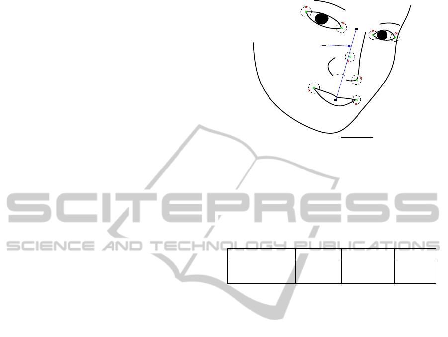
Figure 4: The illustration of two accuracy statistics used

to benchmark the detectors. The green and the red crosses

denote the manually annotated landmarks and the detected

landmarks, respectively. The deviations ε

,.. .,ε

corre-

spond to radii of the dashed circles.

Table 1: The partitioning of the LFW database into training,

validation and testing set.

Data set Training Validation Testing

Percentage 60% 20% 20%

# of examples 6,919 2,307 2,316

L(s,s

) deﬁned by equation (6) and ii) the maximal

normalized deviation

max

(s,

s) = κ(s) max

j=0,...,M−1

−

k, (17)

where s = (s

,. .. ,s

M−1

) are the manually annotated

landmark positions and

s = (

,. .. ,

M−1

) are the

landmark positions estimated by the tested detector.

Figure 4 illustrates both accuracy measures.

4.2 Competing Methods

In this section, we outline all detectors that were used

in the experimental evaluation.

4.2.1 Proposed Detector

The proposed detector estimates the landmark posi-

tions according to the formula (4). As the feature de-

scriptor Ψ

(I,s

) deﬁning the local appearance model

(I,s

), we use the LBP pyramid described in Sec-

tion 2.1. As the parametrization Ψ

i j

) of the de-

formation cost g

i j

), we use the quadratic func-

tion described in Section 2.2. The parameter vec-

tor w of the classiﬁer (4) is trained from the training

part of the LFW database using the BMRM algorithm

(c.f. Section 3.1). The regularization constant λ ap-

pearing in the learning problem (7) was selected from

VISAPP 2012 - International Conference on Computer Vision Theory and Applications

552

the set {10,1,0.1,0.01,0.001} to minimize the aver-

age mean normalized deviation R

VAL

computed on the

validation part of the LFW database.

4.2.2 Independently Trained SVM Detector

This detector is formed by standard two-class linear

SVM classiﬁers trained independently for each land-

mark. For training, we use the SVM solver imple-

mented in LIBOCAS (Franc and Sonnenburg, 2010).

For each individual landmark we created a different

training set containing examples of the positive and

negative class. The positive class is formed by images

cropped around the ground truth positions of the re-

spective component. The negative class contains im-

ages cropped outside the ground truth regions. Specif-

ically, the negative class images satisfy the following

condition



−

− P



width



−

− P



height

where P

−

and P

is the x-coordinate of the neg-

ative and the ground truth component respectively.

height

and width

denote the width and the height

of the component.

We use the LBP-pyramid descriptor (see Sec-

tion 2.1) as the features. The parameters of the linear

SVM classiﬁer are learned from the training part of

the LFW database. The SVM regularization constant

C was selected from the set {10, 1,0.1, 0.01,0.001}

to minimize the classiﬁcation error computed on the

validation part of the LFW database.

Having the binary SVM classiﬁers trained for all

components, the landmark position is estimated by

selecting the place with the maximal response of the

classiﬁer scoring function, evaluated in the search re-

gions deﬁned for each component differently. The

search regions as well as the sizes of the components

are exactly the same as we use for the proposed SO-

SVM detector.

Note that the independently trained SVM detector

is a simple instance of the DPM where the deforma-

tion cost g

i j

) is zero for all positions inside the

search region and −∞ outside. We compare this base-

line detector with the proposed SO-SVM detector to

show that by learning the deformation cost from data

one can improve the accuracy.

4.2.3 Active Appearance Models

We use a slightly modiﬁed version of a publicly avail-

able implementation of the AAM (Kroon, 2010). As

the initial guess of the face position required by the

AAM, we use the center of the bounding box obtained

from a face detector. The initial scale is also com-

puted from this bounding box. The AAM estimates

a dense set of feature points which are distributed

around important face contours like the contour of

mouth, eyes, nose, chin and eyebrows. The AAM

requires a different training database which contains

high resolution images along with annotation of all

contour points.

For training the AAM model we use a publicly

available IIM Face database (Nordstrøm et al., 2004).

The IIM database consists of 240 annotated images

(6 images per person). Each image is 640 × 480 pixel

in size and comes with 58 manually annotated points

which are distributed along the main face contours.

Note that the creation of training examples for the

AAM put much higher demands on the annotator—

he/she has to click a large number of uniformly dis-

tributed points. In contrast, our method requires anno-

tation of only a small number of well deﬁned points.

Speciﬁcally, the whole IIM database requires to an-

notate 13920 points, carefully distributed along each

contour, while the LFW database requires to annotate

48433 points, which are well deﬁned and easy to an-

notate.

To compare the AAM based detector with our de-

tector, we have to transform the output of the AAM,

i.e. the points on contours around important face

parts, to the landmark positions returned by our detec-

tor. We simply select the relevant points on contours.

4.3 Detector of Everingham et al.

The last competing detector is the DPM based detec-

tor of (Everingham et al., 2008). This detector was

trained on a collection of consumer images which,

however, are not available. This detector returns can-

thi of both eyes (4 landmarks), corners of the mouth

(2 landmarks) and 3 landmarks on the nose. To com-

pare this detector, we consider only the relevant land-

marks for our detector. Note that unlike the proposed

SO-SVM detector, this detector learns the local ap-

pearance model and the deformation cost of the DPM

independently.

4.4 Results

In this section, we describe results of the experimental

evaluation of the detection accuracy of all competing

detectors. We have measured the mean and the max-

imal normalized deviation computed on the test part

of the LFW database.

Table 2 shows the average mean normalized de-

viation R

TST

and the the average maximal normal-

ized deviation R

max

TST

for each individual detector. The

results show that the proposed detector consistently

outperforms all other competing methods irrespective

DETECTOR OF FACIAL LANDMARKS LEARNED BY THE STRUCTURED OUTPUT SVM

553

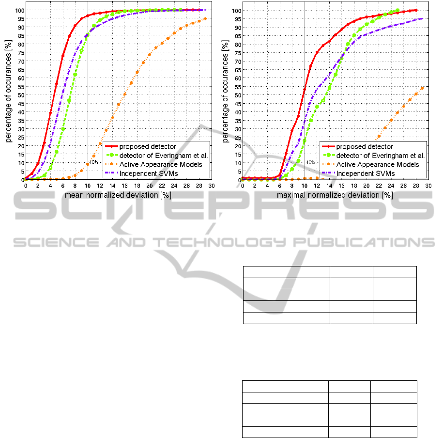
Figure 5: Cumulative histograms for the mean and the maximal normalized deviation shown for all competing detectors.

to the accuracy measure. Surprisingly, the indepen-

dently trained SVM detector is comparable with the

DPM based detector of (Everingham et al., 2008).

The far worst results were obtained for the AAM

based detector which can be attributed to a relatively

low resolution of the input images.

In Figure 5 we show the cumulative histograms of

the mean and maximal normalized deviation. Table 3

shows the percentage of examples from the test part

of the LFW database with the mean/maximal normal-

ized deviation less or equal to 10% (this corresponds

to the line at 10% of x-axis taken from Figure 5. It

is seen that the proposed detector estimates around

97% of images with the mean normalized deviation

less than 10%. This results is far better than was

achieved for all other competing methods. In Fig-

ure 6, we show examples of images with the mean

normalized deviation equal to 10% for better under-

standing of these statistics.

We have also measured the average time required

by the proposed detector to process a single image.

The measurements were done on a notebook with In-

tel Core 2 Duo T9300 2.50 GHz. The average detec-

tion time is 8 ms per image.

4.5 Comparison of BMRM and SGD

In this section, we compare performance of the

BMRM and the SGD algorithm on the problem

emerging when learning the proposed detector. The

task of the solvers is to minimize the problem stated in

(7). Besides the value of the objective function F(w)

of the task (7) we also measured the validation risk

Table 2: Average mean normalized deviation and the av-

erage maximal normalized deviation computed on the test

part of the LFW database.

TST

max

TST

AAM 17.6042 31.2715

Independent SVMs 7.1970 18.3601

Everingham et al. 7.9975 15.9451

proposed detector 5.4606 12.4080

Table 3: The percentage of images from the test part of the

LFW database where the mean/maximal normalized devia-

tion of the estimated landmark positions was less or equal

to 10%.

Mean Maximal

AAM 8.98% 0.62%

Everingham et al. 85.28% 22.93%

binary SVM 85.66% 34.50%

proposed detector 96.59% 53.23%

VAL

(w) being another important criterion character-

izing convergence of the learning algorithm.

To make the iterations of both algorithms compa-

rable, we deﬁne one iteration of the SGD as a se-

quence of single update steps equal to the number

of training examples. This makes the computational

time of both solvers approximately proportional to the

number of iterations. The optimal value of parame-

ter t

for SGD was selected to minimize the objective

function F(w) computed on 10% of the training ex-

amples after one pass of the SGD algorithm thorough

the data. The parameter t

have to be tuned for each

value of λ separately. We ﬁxed the total number of

iterations of the SGD algorithm to 50.

VISAPP 2012 - International Conference on Computer Vision Theory and Applications

554

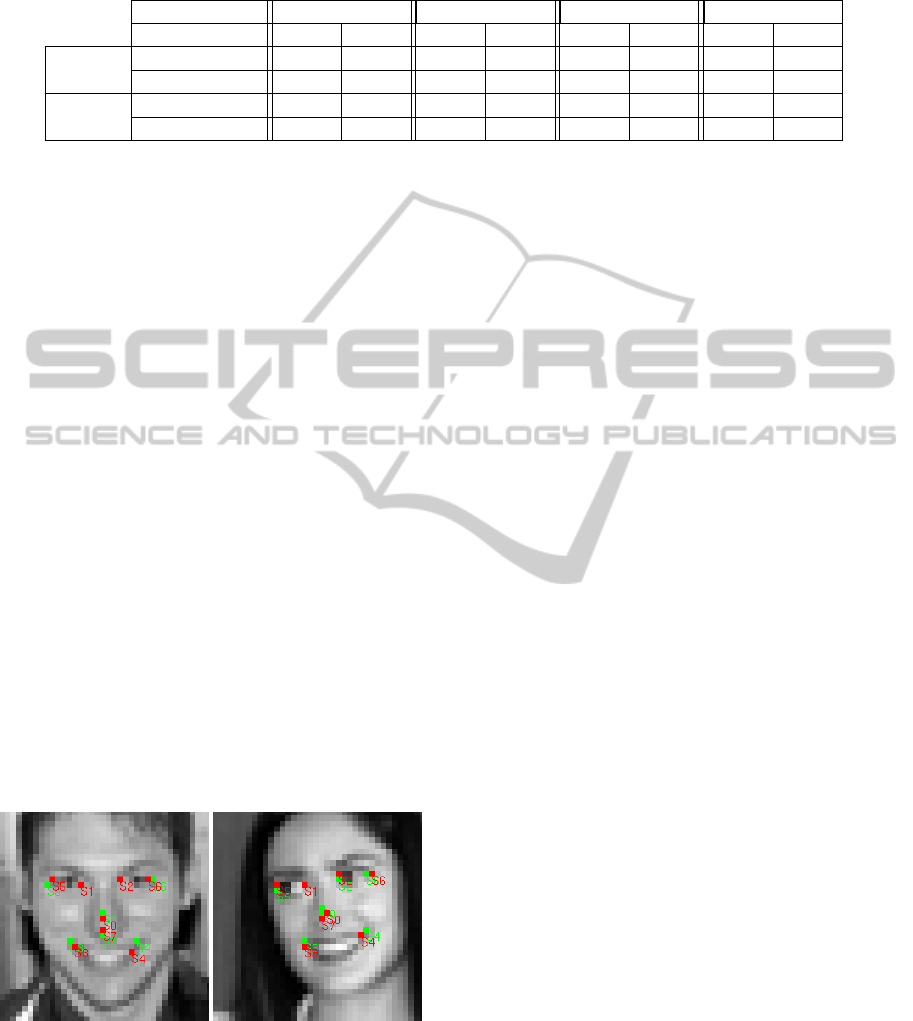
Table 4: Comparison of the BMRM and the SGD. We show the value of primal objective function F(w) and validation risk

VAL

for the 50th iteration (assuming termination of SGD after this iteration) as well as for the number of iterations needed

by the BMRM algorithm to ﬁnd the ε-precise solution.

λ λ = 1 λ = 0.1 λ = 0.01 λ = 0.001

# of iterations 50 106 50 201 50 462 50 1200

BMRM

F(w) 77.48 62.19 45.13 29.68 35.33 14.62 34.35 7.459

VAL

(w) 23.24 10.48 9.054 6.067 9.054 5.475 9.054 5.876

SGD

F(w) 50.88 50.44 20.62 20.52 13.72 10.80 12.86 6.309

VAL

(w) 9.719 9.627 6.156 6.142 5.577 5.496 5.544 5.818

We run both solver on the problem (7) with the

parameters λ ∈ {0.001,0.01,0.1,1} recording both

F(w) and R

VAL

(w). Results of the experiment are

summarized in Table 4.

It can be seen that the SGD converges quickly at

the beginning and it stalls as it approaches the mini-

mum of the objective F. Similarly for the validation

risk. The optimal value of λ minimizing the validation

error was 0.01 for both SGD and BMRM. The test er-

rors computed for the optimal λ were R

TST

= 5.44

for the SGD and R

TST

= 5.54 for the BMRM, i.e.,

the difference is not negligible. The results for the

SGD could be improved by using more than 50 iter-

ations, however, in that case both algorithms would

require the comparable time. Moreover, without the

reference solution provided by the BMRM one would

not know how to set the optimal number of iterations

for the SGD. We conclude that for the tested prob-

lem the BMRM produced more accurate solution, but

the SGD algorithm was signiﬁcantly faster. This sug-

gests that the SGD is useful in the cases when using

the precise but slower BMRM algorithm is prohibited.

In the opposite case the BMRM algorithm returning a

solution with the guaranteed optimality certiﬁcate is

preferable.

(a) (b)

Figure 6: Sample images where the estimated landmark po-

sitions have the mean normalized deviation equal to 10%.

The green and red points denote the manually annotated and

estimated landmarks, respectively.

5 OPEN-SOURCE LIBRARY AND

LFW ANNOTATION

We provide an open-source library which implements

the proposed DPM detector as well as the BMRM

algorithm for learning its parameters from annotated

examples. The detector itself is implemented in C but

we also provide a MEX interface to MATLAB. The

library comes with several example applications writ-

ten in C, e.g. running the detector on still images or on

a video stream from a web camera. The BMRM algo-

rithm is implemented in MATLAB up to time-critical

operations which are in C. The library is licensed un-

der the GNU/GPL version 3 and it was tested under

GNU/Linux and Windows platform.

In addition, we provide a manual annotation

of the LFW database for non-commercial use.

The following set of landmarks is annotated for

each face: the centers of both eyes, canthi for

both eyes, the tip of the nose, the center of the

mouth and the corners of mouth, i.e. 10 anno-

tated landmarks in total for each image. The li-

brary and the annotation can be downloaded from:

http://cmp.felk.cvut.cz/∼uricamic/ﬂandmark

6 CONCLUSIONS

In this paper, we have formulated the detection of fa-

cial landmarks as an instance of the structured output

classiﬁcation problem. Our structured output classi-

ﬁer is based on the DPM and its parameters can be

learned from examples by the SO-SVM algorithm.

In contrast to the previous works, the learning objec-

tive is directly related to the accuracy of the result-

ing detector. Experiments on the LFW database show

that the proposed detector consistently outperforms a

baseline independently trained SVM detector and two

public domain detectors based on the AAM and DPM.

We provide an open-source implementa-

tion of the proposed detector and the manual

annotation of facial landmark for the LFW

DETECTOR OF FACIAL LANDMARKS LEARNED BY THE STRUCTURED OUTPUT SVM

555

database. Both can be downloaded from:

http://cmp.felk.cvut.cz/∼uricamic/ﬂandmark

ACKNOWLEDGEMENTS

The ﬁrst two authors were supported by EC project

FP7-ICT-247525 HUMAVIPS. The second author

was also supported by EC project PERG04-GA-2008-

239455 SEMISOL. The last authors was supported by

the Czech Ministry of Education project 1M0567.

REFERENCES

Beumer, G., Tao, Q., Bazen, A., and Veldhuis, R. (2006).

A landmark paper in face recognition. In 7th In-

ternational Conference on Automatic Face and Ges-

ture Recognition (FGR-2006). IEEE Computer Soci-

ety Press.

Beumer, G. and Veldhuis, R. (2005). On the accuracy of

EERs in face recognition and the importance of re-

liable registration. In 5th IEEE Benelux Signal Pro-

cessing Symposium (SPS-2005), pages 85–88. IEEE

Benelux Signal Processing Chapter.

Bordes, A., Bottou, L., and Gallinari, P. (2009). Sgd-

qn: Careful quasi-newton stochastic gradient descent.

Journal of Machine Learning Research, 10:1737–

1754.

Cootes, T., Edwards, G. J., and Taylor, C. J. (2001). Active

appearance models. IEEE Trans. Pattern Analysis and

Machine Intelligence, 23(6):681–685.

Crandall, D., Felzenszwalb, P., and Huttenlocher, D. (2005).

Spatial priors for part-based recognition using statisti-

cal models. In In CVPR, pages 10–17.

Cristinacce, D. and Cootes, T. (2003). Facial feature de-

tection using adaboost with shape constraints. In

14th Proceedings British Machine Vision Conference

(BMVC-2003), pages 231–240.

Cristinacce, D., Cootes, T., and Scott, I. (2004). A multi-

stage approach to facial feature detection. In 15th

British Machine Vision Conference (BMVC-2004),

pages 277–286.

Erukhimov, V. and Lee, K. (2008). A bottom-up framework

for robust facial feature detection. In 8th IEEE Inter-

national Conference on Automatic Face and Gesture

Recognition (FG2008), pages 1–6.

Everingham, M., Sivic, J., and Zisserman, A. (2006).

“Hello! My name is... Buffy” – automatic naming of

characters in TV video. In Proceedings of the British

Machine Vision Conference.

Everingham, M., Sivic, J., and Zisserman, A. (2008).

Willow project, automatic naming of characters

in tv video. MATLAB implementation, www:

http://www.robots.ox.ac.uk/∼vgg/research/nface/inde

x.html.

Everingham, M., Sivic, J., and Zisserman, A. (2009). Tak-

ing the bite out of automatic naming of characters in

TV video. Image and Vision Computing, 27(5).

Felzenszwalb, P. F., Girshick, R. B., McAllester, D., and

Ramanan, D. (2009). Object detection with discrimi-

natively trained part based models. IEEE Transactions

on Pattern Analysis and Machine Intelligence, 99(1).

Felzenszwalb, P. F. and Huttenlocher, D. P. (2005). Pictorial

structures for object recognition. Internatinal Journal

of Computer Vision, 61:55–79.

Fischler, M. A. and Elschlager, R. A. (1973). The repre-

sentation and matching of pictorial structures. IEEE

Transactions on Computers, C-22(1):67–92.

Franc, V. and Sonnenburg, S. (2010). Libocas —

library implementing ocas solver for training

linear svm classiﬁers from large-scale data. www:

http://cmp.felk.cvut.cz/ xfrancv/ocas/html/index.html.

Heikkil

a, M., Pietik

ainen, M., and Schmid, C. (2009). De-

scription of interest regions with local binary patterns.

Pattern Recognition, 42(3):425–436.

Huang, G. B., Ramesh, M., Berg, T., and Learned-Miller,

E. (2007). Labeled faces in the wild: A database for

studying face recognition in unconstrained environ-

ments. Technical Report 07-49, University of Mas-

sachusetts, Amherst.

Kroon, D.-J. (2010). Active shape model (ASM) and active

appearance model (AAM). MATLAB Central, www:

http://www.mathworks.com/matlabcentral/ﬁleexchan

ge/26706-active-shape-model-asm-and-active-

appearance-model-aam.

Nordstrøm, M. M., Larsen, M., Sierakowski, J., and

Stegmann, M. B. (2004). The IMM face database - an

annotated dataset of 240 face images. Technical re-

port, Informatics and Mathematical Modelling, Tech-

nical University of Denmark, DTU.

Riopka, T. and Boult, T. (2003). The eyes have it. In

Proceedings of ACM SIGMM Multimedia Biometrics

Methods and Applications Workshop, pages 9–16.

Sivic, J., Everingham, M., and Zisserman, A. (2009). “Who

are you?” – learning person speciﬁc classiﬁers from

video. In Proceedings of the IEEE Conference on

Computer Vision and Pattern Recognition.

Teo, C. H., Vishwanthan, S., Smola, A. J., and Le, Q. V.

(2010). Bundle methods for regularized risk mini-

mization. J. Mach. Learn. Res., 11:311–365.

Tsochantaridis, I., Joachims, T., Hofmann, T., Altun, Y.,

and Singer, Y. (2005). Large margin methods for

structured and interdependent output variables. Jour-

nal of Machine Learning Research, 6:1453–1484.

Viola, P. and Jones, M. (2004). Robust real-time face de-

tection. International Journal of Computer Vision,

57(2):137–154.

Wu, J. and Trivedi, M. (2005). Robust facial landmark de-

tection for intelligent vehicle system. In IEEE Inter-

national Workshop on Analysis and Modeling of Faces

and Gestures.

VISAPP 2012 - International Conference on Computer Vision Theory and Applications

556