ROBUST DEFORMABLE MODEL FOR SEGMENTING THE LEFT
VENTRICLE IN 3D VOLUMES OF ULTRASOUND DATA
Carlos Santiago, Jorge S. Marques and Jacinto Nascimento
Institute for Systems and Robotics, Instituto Superior Tecnico, Lisbon, Portugal
Keywords:
3D Echocardiography, Left ventricle, Segmentation, Deformable models, Feature extraction, Robust estima-
tion.
Abstract:
The segmentation of the left ventricle (LV) in echocardiographic data has proven itself a useful methodology
to assess cardiac function and to detect abnormalities. Traditionally, cardiologists segment the LV border at the
end-systolic and end-diastolic phases to determine the ejection fraction. However, the manual segmentation
of the LV is a tedious and time demanding task, which means automated segmentation systems can provide a
powerful tool to improve workflow in a clinical setup. This paper proposes a robust 3D segmentation system
consisting of a deformable model that uses a probabilistic data association filter (PDAF) to robustly detect the
LV border. Results show that the algorithm performs well in both synthetic and real data, without significantly
compromising its performance. The obtained LV segmentations are compared with the manual segmentations
performed by an expert, yielding an average distance of 4 pixel between points from both segmentations.
1 INTRODUCTION
Echocardiography has arguably become amongst the
most preferred medical imaging modality to visualize
the left ventricle (LV). This is mainly due to several
reasons, such as, its low cost and portability(Juang
et al., 2011). The diagnosis usually comprises the
intervention of an expert who manually segments
the LV boundary at the end-systole and end-diastole
phases. This is a necessary step for further quanti-
tative analysis of the heart in order to detect possi-
ble cardiopathies present in the LV. Such procedure is
generally (i) tedious and time consuming, (ii) prone to
errors and (iii) has a significant inter-variability of the
segmentation among specialists. Besides, this image
modality presents several challenges among which we
point out (i) the poor images quality (low SNR ratio),
(ii) the edge dropout specially in the diastole phase,
(iii) the presence of outliers, and (iv) the presence of
multiplicative noise (i.e, Rayleigh), see Fig. 1 for an
illustration. Consequently, only experts are able to
correctly locate the LV boundary.
The above mentioned problems can be alleviated
with the use of an automatic LV segmentation sys-
tem. Initially, automatic LV segmentation systems
were developed for 2D echocardiography. As soon as
the 3D echocardiography became available, methods
to perform the segmentation also became available in
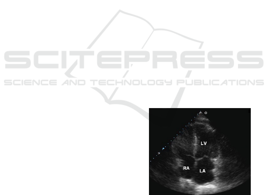
Figure 1: Echocardiography - apical four-chamber view
(Chan and Veinot, 2011).
the literature. One approach to perform 3D segmen-
tation is to consecutively applying 2D segmentations
to each image plane and assembling them into a 3D
structure (Nillesen et al., 2006; Scowen et al., 2000) -
as cardiologists manually do in such cases. However,
such approaches require additional methods to pre-
vent inconsistencies in the surface. Other approaches
have performed the 3D segmentation using the level-
set method, such as in (Juang et al., 2011; Hang et al.,
2005; Yu et al., 2006), and even 3D tracking systems
(Yang et al., 2008; Orderud, 2010).
One of the above mentioned difficulties, is the
presence of outliers, i.e. the invalid features that do
333
Santiago C., S. Marques J. and Nascimento J..
ROBUST DEFORMABLE MODEL FOR SEGMENTING THE LEFT VENTRICLE IN 3D VOLUMES OF ULTRASOUND DATA.
DOI: 10.5220/0003858403330340
In Proceedings of the 1st International Conference on Pattern Recognition Applications and Methods (SADM-2012), pages 333-340
ISBN: 978-989-8425-98-0
Copyright
c
 2012 SCITEPRESS (Science and Technology Publications, Lda.)

not belong to the boundary of the object of inter-
est, in this case, the LV surface. The presence of
outliers should be avoided as far as possible, since
it often leads to meaningless shape estimation re-
sults. To overpass this difficulty, we propose a ro-
bust 3D segmentation algorithm capable of discern-
ing between valid and invalid image features. To
accomplish this, the algorithm is based on a proba-
bilistic data association filter (Bar-Shalom and Fort-
mann, 1988). Two main underlying ideas of the al-
gorithm are as follows. First middle level features
are considered. More specifically, patches are used.
Second, a labeling process (valid-invalid) is assigned
to each patch. Since we do not know beforehand,
the reliability of the patches, all possible labeling se-
quences of valid/invalid patch labels are considered.
Each patch sequence is called here as patch interpre-
tation. Finally, a probability (association probability)
is assigned to each patch interpretation. Thus, in the
adopted strategy, all the patches contribute to the evo-
lution of the deformable model with different weights.
The paper is organized as follows: Section 2
presents an overview of the proposed segmentation
system; Section 3 describes the deformable model
used; Section 4 addresses the feature extraction al-
gorithm and the middle-level features assemblage;
and Section 5 presents the robust model estimation
technique inspired in the S-PDAF algorithm. Sec-
tion 6 shows results of segmentation system applied
to synthetic data and to the segmentation of the LV
in echocardiographic images. Finally, Section 7 con-
cludes the paper with final remarks about the devel-
oped system and future research areas.
2 SYSTEM OVERVIEW
The idea behind of the present approach is to tackle
the difficulties of classic deformable contour methods
associated with noisy images (such as ultrasound im-
ages) by introducing a robust estimation scheme. The
robust framework is inspired in the S-PDAF (Nasci-
mento and Marques, 2004), developed for shape
tracking in cluttered environments. Here we extend
it to the context of 3D shape estimation.
The proposed segmentation system uses a 3D de-
formable model to characterize the surface of the seg-
mentation. This deformable surface requires an ini-
tialization procedure that ensures it is initialized in the
vicinity of the LV boundary.
The adaptation procedure is an iterative process
that consists of the following steps: after initializa-
tion of the model, an adaptation cycle begins with
the detection of low-level features, searched in the
vicinity of the model. Then, these are grouped into
middle-level features (patches). Based on the assem-
bled patches, the S-PDAF algorithm determines all
possible interpretations of considering a patch valid or
invalid and assigns to each patch interpretation a con-
fidence degree that is used to define the estimate of the
boundary location. The model estimate is then used to
fit the surface to the LV boundary, ending an iteration
of the adaptation cycle. The process repeats until the
surface is considered close to the LV boundary. The
following figure shows a diagram of the adaptation
cycle.
Figure 2: Diagram of the proposed segmentation system.
3 SURFACE MODEL
The proposed segmentation system uses a simplex
mesh (Delingette, 1999) as the deformable model. A
3D simplex mesh is a meshed surface composed of
vertices and edges, where each vertex has three neigh-
boring vertices (i.e., belongs to three edges) (see Fig.
4). This particular structure allows to define geo-
metric relations between vertices that are used in the
adaptation procedure to ensure a smooth surface and
good vertices distribution.
3.1 Law of Motion
Each vertex adapts in an iterative process under the
influence of external and internal forces and its final
position is determined by the equilibrium of forces of
the following equation (Delingette, 1999):
P
i
(k+1) = P
i
(k)+(1−γ)(P
i
(k)−P
i
(k−1))+α
i
F
int
i
(k)+β
i
F
ext
i
(k)
(1)
where the parameters γ, α and β are constants.
The internal force, F
int
, is responsible for main-
taining the smoothness of the surface, making use of
the geometric relations between vertices. On the other
hand, the external force, F
ext
, is responsible to attract
each vertex towards the object boundary.
ICPRAM 2012 - International Conference on Pattern Recognition Applications and Methods
334

3.2 Model Initialization
The initialization procedure has to meet the following
conditions: 1) the initial model should be initialized
in the vicinity of the LV boundary; and 2) it should be
a simplex mesh. These two conditions are met using
the following three step procedure.
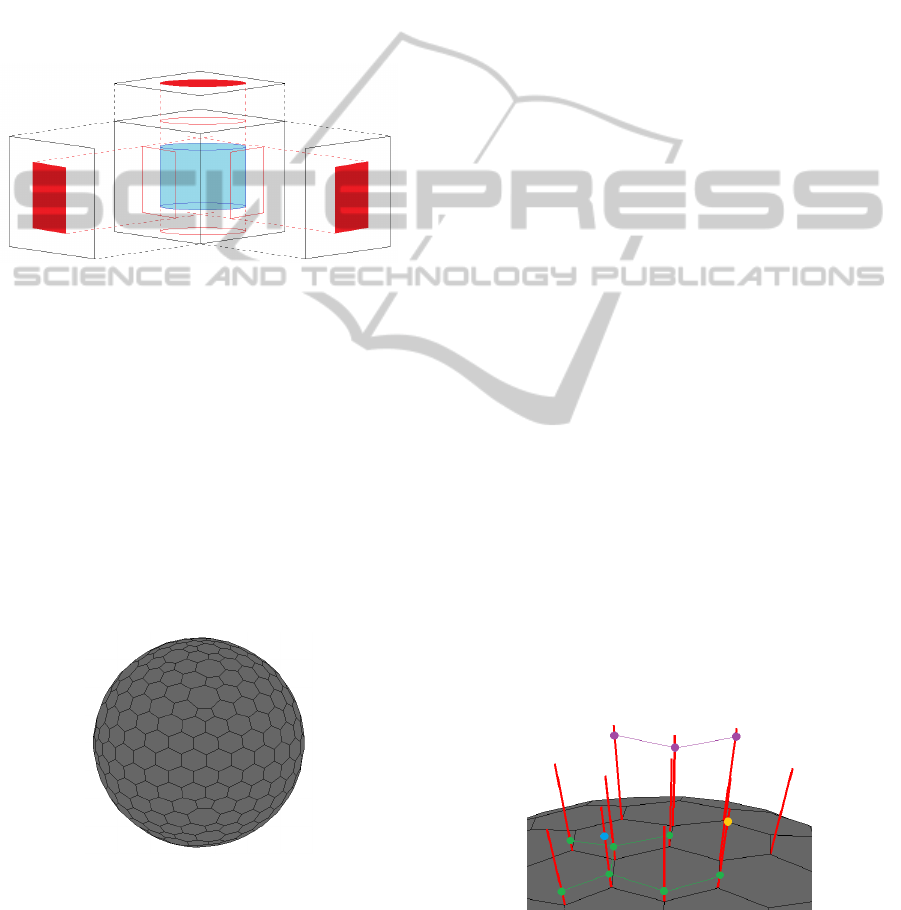
First, to ensure that the model is initialized in the
vicinity of the LV boundary, the user manually defines
a coarse outline of the LV in three orthogonal planes.
A 3D region is then obtained by space carving (Kutu-
lakos and Seitz, 2000) (see Fig. 3).
Figure 3: Schematic example of the computation of the
carved volume (cylinder) (in light blue) by intersection of
the segmented projections (in red).
Second, the simplex mesh is initialized as a sphere
in the center of the carved volume. After uniformly
sampling sphere points, the convex hull algorithm
(Barber et al., 1996) is applied, resulting in a trian-
gular mesh on the sphere surface. Then, taking into
account the duality between simplex meshes and tri-
angulations (Delingette, 1999), an associated simplex
mesh can be formed by considering the center of each
triangle as vertices and linking each vertex with the
center of the three neighboring triangles, resulting in
the simplex mesh shown in Fig. 4.
Figure 4: Simplex mesh initialized as a sphere.
Finally we let the spherical simplex mesh deform
until it fits the carved region. This region corresponds
to the silhouette of the LV boundary and simplifies an
initial adaptation to the dataset since it is a noiseless
binary volume.
4 FEATURE EXTRACTION
The detection of the LV border is performed by the
feature extraction algorithm. First, the volume is pre-
processed using a median filter with a window size
of 4 × 4 pixels. Feature extraction is then performed
using a directional feature search in the vicinity of the
surface model.
4.1 Feature Detection
At each vertex, P
i
, of the simplex mesh, we com-
pute the normal to the surface and define a search line
parallel to the normal vector that passes through P
i
.
Then, the intensity signal along the search line is an-
alyzed. The LV border features are detected using an
edge detector filter, as described in (Blake and Isard,
1998). The filter output’s maxima are extracted us-
ing a threshold and a non-maximum suppression tech-
nique.
Although this methodology has good results,
many undesired features are still detected, depending
on the threshold used. In our experimental setup we
obtained, for each vertex, an average number of fea-
tures that varies from one up to four. Recall that, only
one of these features corresponds to the LV boundary.
4.2 Middle-level Features
To increase the robustness of the feature detec-
tion, these are grouped into middle-level features
(patches). To assemble these patches, we use a label-
ing algorithm that assumes that features should be-
long to the same patch if: 1) the corresponding ver-
tices are neighbors in some level (i.e., the patch is a
connected graph of its features); 2) all features associ-
ated with the same vertex have different labels; and 3)
the distance between neighboring features in a patch
must not exceed a chosen threshold. Fig. 5 shows an
example of the labeling result.
Figure 5: Example of middle-level features. Each color rep-
resents a different patch.
In order to achieve the desired label configura-
tion, L, an energy function is used composed of three
ROBUST DEFORMABLE MODEL FOR SEGMENTING THE LEFT VENTRICLE IN 3D VOLUMES OF
ULTRASOUND DATA
335

terms:
E(L) = E
1
(L) + E
2
(L) + E
3
(L) (2)
This energy is computed as a sum of the energy of
each individual label.
The first term, E
1
(L), is minimum when features
with the same label are the closest features associ-
ated with the neighboring vertices. The second term,
E
2
(L), prevents patches from having features too far
apart. This is done by assigning an energy of ∞ to la-
bels where the distance between neighboring features
exceeds the labeling threshold. If the distance is lower
than the threshold, the energy yields the value 0. Fi-
nally, the third term, E
3
(L), prevents repeated labels
in features associated with the same vertex, again as-
signing an energy value of ∞ if this occurs and 0 oth-
erwise.
The label configuration L that minimizes the total
energy function (2) corresponds to the configuration
that obeys all the conditions.
The energy minimization algorithm uses a region
growing scheme where a label is seeded in a random
feature and it propagates to the surrounding features
whenever an energy decrease is possible. This pro-
cess repeats until all features have been labeled. The
pseudocode in Table 1 describes the developed label-
ing algorithm:
Table 1: Labeling algorithm.
Q = {} % labeling queue
C = {} % labeled features
repeat
If Q is empty
seed a new label l in a random feature y
i
/∈ C
add y
i
to C
for each feature y
k
neighbor of y
i
if y
k
/∈ C & labeling y
k
with l lowers E(L)
add y
k
to Q
Else
repeat
y
i
= Q(1)
label y
i
with l
add y
i
to C
remove y
i
from Q
for each feature y
k
neighbor of y
i
if y
k
/∈ C & labeling y
k
with l lowers E(L)
add y
k
to Q
until Q is empty
until all features have been labeled
The size of the resulting patches and their distance
to the surface provides good differentiation measures
to assess if the features in that patch belong to the LV
boundary or if they were produced by the background.
5 ROBUST MODEL ESTIMATION
The robust model estimation used is an extension of
the S-PDAF algorithm described in (Nascimento and
Marques, 2004) to the 3D case. In each iteration k,
this estimation technique considers all possible com-
binations of considering each patch as valid or in-
valid. Assuming M
k
patches were detected, there
are m
k
= 2
M
k
possible interpretations. Each com-
bination is defined as a patch interpretation I
i
(k) =
{I
1
i
(k), .. .,I
n
i
(k), .. .,I
M
k
i
(k)}, where I
n
i
(k) = 0 if the
nth patch in the ith interpretation is considered invalid
and I
n
i
(k) = 1 otherwise.
The model assumes that the LV boundary position
is described by
x(k) = x(k − 1) + w(k) (3)
where w(k) ∼ N(0,Q) is white Gaussian noise with
normal distribution.
For each interpretation I
i
(k), the observations
y
i
(k) are generated by a different model. If an obser-
vation y
i
(k) is considered invalid (outlier), the model
assumes it is generated by uniform distribution. Oth-
erwise, the model assumes it relates to the boundary
points x(k) by:
y
i
(k) = x(k) + v
i
(k) (4)
where v
i
(k) ∼ N(0, R
i
) is a white Gaussian noise with
normal distribution associated with the valid features
y
i
(k) of the interpretation I
i
(k).
The state estimate is then defined by:
ˆx(k) =
m
k
∑
i=0
ˆx
i
(k)α
i
(k) (5)
where ˆx
i
(k) is the updated state conditioned on the hy-
pothesis that I
i
(k) is correct (which is the same as the
update state equation of a traditional Kalman filter),
and α
i
(k) is the association probability of the interpre-
tation I
i
(k). A similar analysis is done to predict and
update the covariance matrix (Nascimento and Mar-
ques, 2004).
5.1 Association Probabilities
The association probabilities, α
i
(k), define the
strength of the corresponding interpretation I
i
(k) in
each iteration k of the adaptation procedure (from this
point on we omit the dependence of k for the sake of
simplicity). It is defined as
α
i
= P(I
i
|Y,L, ˆx) (6)
ICPRAM 2012 - International Conference on Pattern Recognition Applications and Methods
336

where Y and L are the set of the detected features
and patches, respectively. Using a Bayesian approach,
this probability can be decomposed into:
α
i
=
P(Y |I
i
,L, ˆx) × P(I
i
|L, ˆx)
β
(7)
where β = P(Y |L, ˆx) is a normalization constant that
does not depend on I
i
, P(Y |I
i
,L, ˆx) is the likelihood
of the set of features Y and P(I
i
|L, ˆx) is the prior
probability of the interpretation I
i
conditioned on the
patches (i.e., based on its valid and invalid patches).
Note that interpretations with overlapping patches
will be assigned an association probability of 0, and
patches considerably smaller then the larger ones will
be promptly discarded to avoid an exponential growth
of possible interpretations.
Assuming that the patches are independently gen-
erated, the likehood P(Y |I
i
,L, ˆx) is expressed as the
product of each individual probability of having a
patch l
n
at an average distance d to the surface. How-
ever, this probability is dependent on the hypothesis
that l
n
is considered valid or invalid: if I
n
i
= 0 it is
assumed that the probability distribution is uniform
along the search line, whereas if I
n
i
= 1 the probability
distribution is assumed Gaussian with mean 0 and co-
variance proportional to the length of the search line,
V . Formally:
P(l
n
|I
i
,L, ˆx) ∼

V
−1
if I
n
i
= 0
ρ
−1
N(d; 0,σ) otherwise
(8)
where ρ is the normalization constant.
As to the prior probability of each interpretation
I
i
, it is related to the size of its valid and invalid
patches. The probability P(I
i
|L, ˆx) is also decomposed
as the product of each individual probability of the
patches, P(I
n
i
|L, ˆx). It is assumed that larger patches
are more likely to belong to the LV boundary. There-
fore, these should receive a higher probability. On the
other hand, when considered invalid, these should be
assigned a small probability.
The resulting prior probability yields:
P(I
i
|L, ˆx) =
∏
l
n
:I
n
i
=1
[alog(A
l
n
+ 1) + b] ×
∏
l
n
:I
n
i
=0
1 − [a log(A
l
n
+ 1) + b)] (9)
where:
a =
P
A
−P
B
1−log(A
max
+1)
b = P
B
− a log(A
max
+ 1).
(10)
and P
A
, P
B
and A
max
are constants, and A
l
n
is the
area of the patch l
n
(number of features it comprises).
These assumptions assure that patches above a certain
area A are preferably considered.
6 RESULTS
The proposed system was tested using several differ-
ent datasets, both real and synthetic. The purpose of
the synthetic data was to assess the functionality of
the model, for which we will present more insight of
the framework. The real data corresponds to echocar-
diographic volumes (courtesy of Dr. Jacinto Nasci-
mento). The algorithm was applied to four different
echocardigraphic volumes. A quantitative assessment
of the system’s performance will be provided using
error metrics between the obtained segmentation and
the manual segmentation performed by an expert - the
ground truth (GT).
6.1 Evaluation Metrics
We use four similarity metrics to compare the output
of the algorithm with the reference contours, namely:
the Hammoude metric (Hammoude, 1988), d
HMD
, the
average metric, d
AV
, the Hausdorff metric (Hutten-
locher et al., 1993), d
HDF
, and mean absolute distance
metric, d
MAD
. These are defined as follows: consider
R
Ψ
as the region delimited by model segmentation
and R
Ω
as the region delimited by the GT. The Ham-
moude metric is defined by:
d
HMD
(Ψ,Ω) =
#((R
Ψ
∪ R
Ω
) − (R
Ψ
∩ R
Ω
)
#((R
Ψ
∪ R
Ω
))
(11)
This error metric corresponds to the fraction of area
between the two contours using a XOR operator. Low
values of d
HMD
indicate high similarity between both
regions.
Now consider the border of the model segmenta-
tion defined by the points Ψ = {ψ
1
,. ..,ψ
N
ψ
} and the
border of the GT Ω = {ω
1
,. ..,ω
N
ω
}. The average
metric between two contours is defined as the average
distance between each point ψ
i
to the closest point in
Ω, d(ψ
i
,Ω) = min
j
||ω
j
− ψ
i
||,
d
AV
=
1
N
Ψ
N
Ψ
∑
i=1
d(ψ
i
,Ω) (12)
where N
Ψ
is the length of Ψ. The Hausdorff metric
is defined as the maximum value of d(ψ
i
,Ω) between
the two contours:
d
HDF
(Ψ,Ω) = max

max
i
{d(ψ
i
,Ω)}, max
j
{d(ω, Ψ)}

(13)
Finally, the MAD metric is defined by:
d
MAD
(Ψ,Ω) =
1
N
N
∑
i=1
||ψ
i
− ω
i
|| (14)
which corresponds to the maximum absolute dis-
tance’s average between corresponding points in the
boundaries.
ROBUST DEFORMABLE MODEL FOR SEGMENTING THE LEFT VENTRICLE IN 3D VOLUMES OF
ULTRASOUND DATA
337

6.2 Parameter Definition
All the presented results were obtained using the pa-
rameters that achieve better overall results:
• In (1), we used α = 0.7, β = 0.05 and γ = 0.9; the
stopping criterion was the average displacement
of the vertices k
stop
< 0.005;
• In the feature extraction algorithm, the thresh-
old using the maxima detection was t
f
= 0.5c
max
,
where c
max
is the highest peak of the filter out-
put; as to the labeling threshold (i.e., the maxi-
mum distance allowed between neighboring fea-
tures with the same label) used was t
l
= 8;
• Finally, in (9) we used P
A
= 0.05, P
B
= 0.95 and
A
max
= 700 (the number of vertices in the surface).
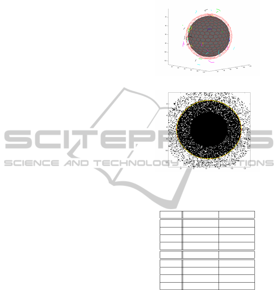
6.3 Synthetic Data
We will present one particular test using a synthetic
volume. This synthetic volume contains a sphere cor-
rupted by white Gaussian noise with zero mean (see
Fig. 7). Although many features are detected (an av-
erage of approximately 3 features associated with a
single vertex), only one large patch is extracted (see
Fig. 6) and all the other smaller noise-originated
patches are discarded. The association probabilities
of the existing interpretations are the following:
α
1
= P(I
1
= {I
1
= 0}) = 0.04
α
2
= P(I
2
= {I
1
= 1}) = 0.96
which means a high confidence degree is assigned to
the large (correct) patch. Fig. 7 shows that the model
is able to correctly adapt to the desired sphere.
6.4 Echocardiographic Data
As mentioned before, the segmentations of the LV
in four different echocardiographic volumes are pre-
sented in Fig. 8. For each volume, a single slice is
shown twice: one containing the obtained segmen-
tation and one containing the GT. The final three-
dimensional surface is also presented.
6.5 Quantitative Assessment
Although the previous results show that the devel-
oped segmentation system performs reasonably well,
quantification measurements are required to compare
its performance with other similar methods. Table 2
presents the values of the similarity metrics.
The table shows high similarity between the esti-
mated contour and the GT, indicating a good match.
Figure 6: Patch detection in a synthetic noisy sphere.
Figure 7: Slice view of the final configuration of the surface
(yellow contour).
Table 2: Results of the evaluation methods for each volume
(the distance values are expressed in pixels).
Volume 1 Volume 2
¯
d
HMD
0.15 ± 0.03 0.20 ± 0.10
¯
d
AV
3.8 ± 0.7 3.1 ± 1.3
¯
d
HDF
11.2 ± 2.5 8.7 ± 3.2
¯
d
MAD
5.5 ± 1.3 4.7 ± 2.8
Volume 3 Volume 4
¯
d
HMD
0.16 ± 0.02 0.24 ± 0.04
¯
d
AV
3.3 ± 0.6 4.6 ± 0.7
¯
d
HDF
8.4 ± 2.1 13.7 ± 2.3
¯
d
MAD
4.4 ± 1.1 8.1 ± 2.5
7 CONCLUSIONS
This paper addresses the automatic LV segmentation
problem in 3D echocardiographic data. Due to the
nature of the volumes, many of the detected fea-
tures usually do not belong to the LV boundary. The
proposed system uses a robust estimation technique
based on PDAF that prevents the segmentation to be
misguided by those outliers.
The results shown demonstrate that the proposed
system performs a good segmentation of the LV, with
potential application to accurately compute cardiac
ICPRAM 2012 - International Conference on Pattern Recognition Applications and Methods
338

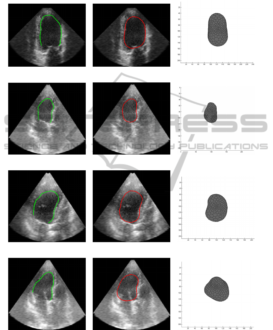
Volume 1
Volume 2
Volume 3
Volume 4
Figure 8: Slice from the echocardiographic showing (on the left) the GT and (on the center) the obtained segmentation. Final
configuration of the surface (on the right).
measurements such the systemic and diastolic vol-
umes and the corresponding ejection fraction.
Further tests shows that the developed system is
slightly over-dependent on the initialization proce-
ROBUST DEFORMABLE MODEL FOR SEGMENTING THE LEFT VENTRICLE IN 3D VOLUMES OF
ULTRASOUND DATA
339

dure, which does not help improving the repeatabil-
ity of LV segmentations. This could be avoided using
an automatic initialization scheme, such as in (Yang
et al., 2008).
ACKNOWLEDGEMENTS
This work was supported by project [PTDC/EEA-
CRO/103462/2008] (project HEARTRACK) and
FCT [PEst-OE/EEI/LA0009/2011].
REFERENCES
Bar-Shalom, Y. and Fortmann, T. (1988). Tracking and
Data Associaton. New York: Academic.
Barber, C. B., Dobkin, D. P., and Huhdanpaa, H. (1996).
The quickhull algorithm for convex hulls. ACM Trans-
actions on Mathematical Software, 22(4):469–483.
Blake, A. and Isard, M. (1998). Active Contour. Springer.
Chan, K.-L. and Veinot, J. P. (2011). Anatomic Basis
of Echocardiographic Diagnosis. Oxford Univesity
Press, 1
st
edition.
Delingette, H. (1999). General object reconstruction based
on simplex mesh. International Journal of Computer
Vision, (32):111–142.
Hammoude, A. (1988). Computer-assisted Endocar-
dial Border Identification from a Sequence of Two-
dimensional Echocardiographic Images. PhD, Uni-
versity Washington.
Hang, X., Greenberg, N., and Thomas, J. (2005). Left ven-
tricle quantification in 3d echocardiography using a
geometric deformable model. Computers in Cardiol-
ogy, pages 649–652.
Huttenlocher, D. P., Klanderman, G. A., and Rucklidge,
W. J. (1993). Comparing images using hausdorff dis-
tance. IEEE Trans. Pattern Anal. Machine Intell.,
15(9):850–863.
Juang, R., McVeigh, E., Hoffmann, B., Yuh, D., and
Burlina, P. (2011). Automatic segmentation of the
left-ventricular cavity and atrium in 3d ultrasound us-
ing graph cuts and the radial symmetry transform. In
2011 IEEE International Symposium on Biomedical
Imaging: From Nano to Macro, pages 606–609.
Kutulakos, K. N. and Seitz, S. M. (2000). A theory of shape
by space carving. International Journal of Computer
Vision, (38):199–218.
Nascimento, J. C. and Marques, J. S. (2004). Robust shape
tracking in the presence of cluttered background.
IEEE Trans. Multimedia, 6(6).
Nillesen, M., Lopata, R., and et al. (2006). 3d segmentation
of the heart muscle in real-time 3d echocardiographic
sequences using image statistics. IEEE Ultrasonics
Symposium, 2006, pages 1987–1990.
Orderud, F. (2010). Real-time segmentation of 3D echocar-
diograms using a state estimation approach with de-
formable models. PhD thesis, Norwegian University
of Science and Technology, Department of Computer
and Information Science.
Scowen, B., Smith, S., and Vannan, M. (2000). Quantita-
tive 3d modelling of the left ventrical from ultrasound
images. In Euromicro Conference, volume 2, pages
432–439.
Yang, L., Georgescu, B., Zheng, Y., Meer, P., and Comani-
ciu, D. (2008). 3d ultrasound tracking of the left ven-
tricle using one-step forward prediction and data fu-
sion of collaborative trackers. In IEEE CVPRW’08,
pages 1–8.
Yu, H., Pattichis, M., and Goens, M. (2006). Robust seg-
mentation and volumetric registration in a multi-view
3d freehand ultrasound reconstruction system. In AC-
SSC ’06, pages 1058–6393.
ICPRAM 2012 - International Conference on Pattern Recognition Applications and Methods
340