AUTOMATIC SELECTION OF THE TRAINING SET FOR

SEMI-SUPERVISED LAND CLASSIFICATION AND

SEGMENTATION OF SATELLITE IMAGES

Olga Rajadell and Pedro Garc´ıa-Sevilla

Institute of New Imaging Technologies, University Jaume I, Castell´on de la Plana, Spain

Keywords:

Semi-supervised classiﬁcation, Image segmentation, Hyper-spectral imaging, Mode seek clustering.

Abstract:

Different scenarios can be found in land classiﬁcation and segmentation of satellite images. First, when prior

knowledge is available, the training data is generally selected by randomly picking samples within classes.

When no prior knowledge is available the system can pick samples at random among all unlabeled data, which

is highly unreliable, and ask the expert to label them or it can rely on the expert collaboration to improve

progressively the training data applying an active learning function. We suggest a scheme to tackle the lack of

prior knowledge without actively involving the expert, whose collaboration may be expensive. The proposed

scheme uses a clustering technique to analyze the feature space and ﬁnd the most representative samples for

being labeled. In this case the expert is just involved in labeling once a reliable training data set for being

representative of the features space. Once the training set is labeled by the expert, different classiﬁers may be

built to process the rest of samples. Three different approaches are presented in this paper: the result of the

clustering process, a distance based classiﬁer, and support vector machines (SVM).

1 INTRODUCTION

The classiﬁcation and segmentation of land usage in

satellite images generally requires an expert who pro-

vides the corresponding labels for the different ar-

eas in the images. Some authors work with prior

knowledge in a supervised scenario and training data

is selected within each class (Y.Tarabalka et al.,

2010)(A.Plaza and et al., 2009). Lately the research

interest in active learning techniques, which move

to a semi-supervised scenario, is raising. In new

real databases, the expert labeling involves whether

prior knowledge or checking at the land place itself,

which could be highly expensive. The expert col-

laboration may be needed an unknown number of

steps to improve the classiﬁcation by helping in the

training selection until the convergence condition is

achieved (Tuia et al., 2009)(Li et al., 2010). Hence,

the expert collaboration can be highly expensive and

picking at random among the unlabeled pool is not

convenient because classes are often very unbalanced

and the probabilities of getting an efﬁcient represen-

tative training data is inverse to the amount of labeled

samples. Consequently, decreasing the size of labeled

data is a problem. To tackle this, the most interest-

ing samples should be provided to the expert from the

beginning (Comaniciu and Meer, 2002).

In unsupervised scenarios, data analysis tech-

niques have proved being good at providing relevant

data when no prior knowledge is available. Among

them, clustering techniques allow us to divide data

in groups of similar samples. Specially when sam-

ples represent pixels from an image, clustering algo-

rithms have successfully been applied to image seg-

mentation in various ﬁelds and applications (Arbe-

laez et al., 2011). We aim to segment and classify

hyper-spectral satellite images. Fully unsupervised

procedures often have insufﬁcient accurate classiﬁca-

tion results. For such a reason, a hybrid scenario be-

tween supervised and unsupervised techniques is our

target where the methods applied could take into ac-

count some labels to build a classiﬁer. We suggest

to use a clustering analysis to ﬁnd samples of inter-

est, ask an expert for their labels and classify using

that labeled set obtained. This scheme was presented

in (Rajadell et al., 2011) where a KNN1 classiﬁer

was used. Here we suggest to assign labels to un-

labeled samples according to the result given by the

cluster itself and the labels provided by the expert for

the modes of clusters. We also adapt and extend the

method in order to be used with SVM. These new seg-

mentation approaches provide interesting results. For

412

Rajadell O. and García Sevilla P..

AUTOMATIC SELECTION OF THE TRAINING SET FOR SEMI-SUPERVISED LAND CLASSIFICATION AND SEGMENTATION OF SATELLITE

IMAGES.

DOI: 10.5220/0003855504120418

In Proceedings of the 1st International Conference on Pattern Recognition Applications and Methods (PRARSHIA-2012), pages 412-418

ISBN: 978-989-8425-98-0

 2012 SCITEPRESS (Science and Technology Publications, Lda.)

all cases, the suggested scheme is compared with the

supervised state of the art classiﬁcation, resulting in

outperforming previous works.

A review of the sample selection scheme with its

spatial improvement is presented in Section 2. Sev-

eral classiﬁcation alternatives are presented in Section

3. Results will be shown and analyzed in Section 5.

Finally, Section 6 presents some conclusions.

2 PRELIMINARIES

Nowadays, due to the improvement in the sensors,

databases used for segmentation and classiﬁcation of

hyper-spectral satellite images are highly reliable in

terms of spectral and spatial resolution. Therefore,

we can consider that our feature space representation

of the data is also highly reliable. On the other hand,

in segmentation and classiﬁcation of this kind of im-

ages the training data used has not been a concerned

so far, without worrying about providing the most re-

liable information (Comaniciu and Meer, 2002). The

scheme suggested in (Rajadell et al., 2011) was a ﬁrst

attempt in this sense. It was proposed an unsupervised

selection of the training samples based on the analysis

of the feature space to provide a representative set of

labeled data. It proceeds as follows:

1. In order to reduce the dimensionality of the prob-

lem, a set of spectral bands, given a desired num-

ber, is selected by using a band selection method.

The WaLuMi band selection method (Mart´ınez-

Us´o et al., 2007) was used in this case, although

any other similar method could be used.

2. A clustering process is used to select the most rep-

resentative samples in the image. In this case,

we have used the Mode Seek clustering procedure

which is applied over the reduced feature space.

An improvement in the clustering process is in-

cluded by adding the spatial coordinates of each

pixel in the image as additional features. Since

the clustering is based on distances, spatial coor-

dinates should also be taken into account assum-

ing the class connection principle.

3. The modes (centers of the clusters) resulting of

the previous step deﬁne the training set for the

next step. The expert is involvedat this point, only

once, by providing the corresponding labels of the

selected samples.

4. The classiﬁcation of the rest of non-selected sam-

ples is performed, using the training set deﬁned

above to build the classiﬁer. Three different clas-

siﬁcation experiments have been performed here:

a KNN classiﬁer with k = 1, a direct classiﬁcation

with the results of the clustering process, and an

extension will be presented for the use of SVM.

2.1 Mode Seek Clustering

Given a hyper-spectral image, all pixels can be con-

sidered as samples which are characterized by their

corresponding feature vectors (spectral curve). The

set of features deﬁned is called the feature space

and samples (pixels) are represented as points in that

multi-dimensional space. A clustering method groups

similar objects (samples) in sets that are called clus-

ters. The similarity measure between samples is de-

ﬁned by the cluster algorithm used. A crucial problem

lies in ﬁnding a good distance measure between the

objects represented by these feature vectors. Many

clustering algorithms are well known. A KNN mode

seeking method will be used in this paper (Cheng,

1995). It selects a number of modes which is con-

trolled by the neighborhood parameter (s). For each

class object x

, the method seeks the dissimilarity to

its s

neighbors. Then, for the s neighbors of x

the dissimilarities to their s

neighbors are also com-

puted. If the dissimilarity of x

to its s

neighbor is

minimum compared to those of its s neighbors, it is

selected as prototype. Note that the parameter s only

inﬂuences the scheme in a way that the bigger it is the

less clusters the method will get since more samples

will be grouped in the same cluster, that is, less modes

will be selected as a result. For further information

about the mode seek clustering method see (Cheng,

1995) and (Comaniciu and Meer, 2002)

2.2 Spatial Improvement

The clustering algorithm searches for local density

maxima where the density function has been calcu-

lated using the distances for each sample in its s

neighborhood using a dissimilarity measure as the

distance between pairs of samples. In that difference,

all features (dimensions) are considered. When fea-

tures do not include any spatial information the class

connection principle is missed (pixels that lie near

in the image are likely to belong to the same class).

Therefore, we suggest to include the spatial coordi-

nates among the feature of the samples. See Fig 1.(a)

where all samples have been represented in the three

ﬁrst features space and in different color per class.

Notice that, when no spatial data is considered and

all classes are located in the same space and when

no prior knowledge is available for the clustering pro-

cess, ﬁnding representatives for each class would be

difﬁcult since the classes themselves may lie together.

Moreover, different areas of the same class may be

AUTOMATIC SELECTION OF THE TRAINING SET FOR SEMI-SUPERVISED LAND CLASSIFICATION AND

SEGMENTATION OF SATELLITE IMAGES

413

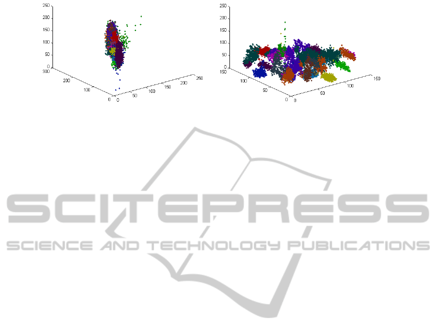
a b

Figure 1: Effects of including spatial information in the feature space. Plots show the samples of the database in the feature

space, colored per class according to the ground-truth. (a) no spatial information is available. (b) spatial coordinates are

included.

within the same cloud. However, when spatial data is

included, Fig 1.(b), the single cloud of samples is bro-

ken according to spatial distances and classes (ﬁelds)

are more separable. In this sense also samples belong-

ing to the same class but lying in different places of

the image are separable.

In (Rajadell et al., 2011) it was suggested to weigh

the spatial coordinates by an arbitrary number to re-

inforce two samples that are close spatially to have

a closer distance and the way round. Such a weight

should be decided in terms of the range of the fea-

tures provided by the spectrometer so the coordinates

are overweighed but they do not cause the rest of fea-

tures be dismissed in the global measure.

3 CLASSIFICATION

ALTERNATIVES

The whole dataset was ﬁrst reduced to 10 bands us-

ing the band method selection named in Section 2.

This method is used for minimizing the correlation

between features but maximizing the amount of infor-

mation provided, all that without changing the feature

space. Clustering was carried out tuning the param-

eter s to get a preﬁxed number of selected samples.

Three different classiﬁcation alternatives have been

used.

3.1 Straightforward Schemes

1. First a KNN with k=1 classiﬁcation has been per-

formed with the labeled samples as training set.

This is not an arbitrary choice, because the clus-

tering procedure used is based on densities calcu-

lated on a dissimilarity space, and therefore, the

local maxima correspond to samples which mini-

mize its dissimilarity with a high amount of sam-

ples around it. Thus, the selected samples are

highly representative in distance-based classiﬁers.

2. Second, another classiﬁcation process has been

performed using the straightforward result of the

clustering procedure. The expert labels the se-

lected samples. Then, all samples belongingto the

cluster that each labeled sample is representing

are automatically labeled in the same class. This

provides a very fast pixel classiﬁcation scheme as

the clustering result is already available.

3.2 Extension to SVM

The scheme, as it has been presented, is not useful for

classiﬁers that are not based on distances. However,

we would like to check if providing relevant train-

ing data may be also useful for other classiﬁers. In

this case, we extend the proposed method for SVM.

For such a classiﬁer, it is interesting to detect samples

in the borders between clusters and not their centers

to achieve representing the shape of the data in the

feature space. Nevertheless, we do not want to in-

crease the amount of labeled data. According to these

criteria we propose selecting samples from the clus-

ter, assuming that those samples have the same label

that the cluster was given. It would be possible to

take the whole cluster itself with the assumed label

as training data but, depending on the database size,

it would not be computationally affordable. On one

hand, using the most distant samples from the clus-

ter center would introduce an important amount of

outliers in the construction of the classiﬁer. On the

other hand, using the samples around the cluster cen-

ter would not help the SVM to ﬁnd the shape of the

cluster. Therefore, two thresholds α

and α

of the

maximum distance inside each cluster has been con-

sidered. Samples between α

and α

are selected for

training the SVM (see Fig 2). Although the amount of

samples selected is higher than the number of modes,

notice that these samples are not labeled by the expert

and, consequently, the number of the labeled samples

ICPRAM 2012 - International Conference on Pattern Recognition Applications and Methods

414

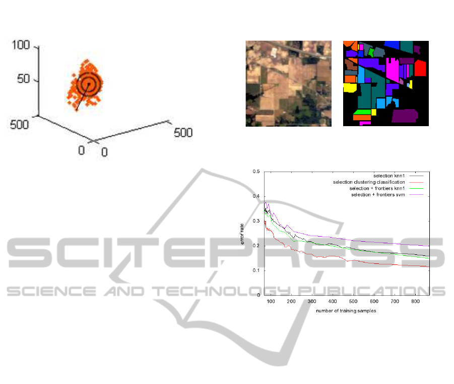
Figure 2: Training selection example for extension of the

scheme to SVM necessities. The samples between α

and

will be used to construct the SVM.

is still the same. However, the real size of the training

set is larger and it should be more representative of

the shape of the data. With this larger set we can train

a SVM and use it to classify the whole image. The use

of these samples would also be possible for the case of

the KNN classiﬁer. However, it is important to point

out that the errors made by the clustering process in

these samples are now introduced in the training set.

4 DATABASE

A well-known database has been used in the exper-

iments (see Fig 3). Hyper-spectral image 92AV3C

was provided by the Airborne Visible Infrared Imag-

ing Spectrometer (AVIRIS) and acquired over the In-

dian Pine Test Site in Northwestern Indiana in 1992.

From the 220 bands that composed the image, 20 are

usually ignored (the ones that cover the region of wa-

ter absorption or with low SNR) (Landgrebe, 2003).

The image has a spatial dimension of 145 × 145 pix-

els. Spatial resolution is 20m per pixel. Classes range

from 20 to 2468 pixels in size. In it, three different

growing states of soya can be found, together with

other three different growing states of corn. Woods,

pasture and trees are the bigger classes in terms of

number of samples (pixels). Smaller classes are steel

towers, hay-windrowed, alfalfa, drives, oats, grass

and wheat. In total, the dataset has 16 labeled classes

and unlabeled part which is known as the background.

This so called background will be here considered as

the 17 class for the segmentation experiments.

5 EXPERIMENTAL RESULTS

In Fig 4 the results obtained using several classiﬁ-

cation strategies are compared: KNN using only the

center of the clusters for the training set, SVM, KNN

Figure 3: 92AV3C AVIRIS database. Color composition

and ground-truth.

Figure 4: Learning curve in terms of error rate when in-

creasing the size of training data in number of samples se-

lected by the scheme suggested. Different classiﬁcation

methods tested using the 92AV3C database.

using the same training set used for the SVM, and the

classiﬁcation using the plain output of the mode seek

clustering. It was already shown in (Rajadell et al.,

2011) that the scheme used with KNN clearly outper-

formed the random selection. Now, the classiﬁcation

result for the KNN classiﬁer adding more samples in

the clusters assuming the same label is very similar

to the ones obtained with the KNN classiﬁer using

only the cluster centers. For SVM the thresholds used

here were α

= 0.3 and α

= 0.4, although several

combinations of values were used providing similar

results in all cases. The SVM classiﬁer provided the

worst results in all experiments. This may be due to

the fact that the double threshold scheme proposed as-

sumes a spherical distribution of the samples around

the cluster centers. However, this is not the case in

general, and that is the reason why SVM cannot prop-

erly model the borders of the classes using these train-

ing samples. On the other hand, the mode seek clus-

tering classiﬁcation outperformed all other methods.

The reason is that this sort of clustering is not based

on the distance to a central sample in the cluster but

to the distance to other samples in the clusters. When

the distance to a central point is considered, a spheric

distribution of the pixels around this point is assumed.

However, the mode seek clustering provides clusters

AUTOMATIC SELECTION OF THE TRAINING SET FOR SEMI-SUPERVISED LAND CLASSIFICATION AND

SEGMENTATION OF SATELLITE IMAGES

415

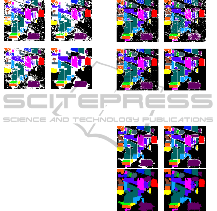
(a) (b)

Figure 5: Segmentation-classiﬁcation results using 0.33%

of data for the selected training set using several classiﬁers.

(a) KKN using the cluster centers. (b) SVM (c) KNN using

the same training set as for the SVM (d) mode seek cluster-

ing.

that may adapt to different shapes, depending on the

distribution of the samples in the feature space, and

these clusters can be modeled using just one sample.

The database has 21025 samples. Fig. 5 show the

classiﬁcation results of several classiﬁers when 0.33%

of the pixels in the image (69 pixels) was labeled

by the expert. The classiﬁcation errors are shown

as white pixels. It can be noted that the clustering

classiﬁer outperformed the other classiﬁers not only

in the percentage of classiﬁcation rate but also pro-

viding smooth compact regions in the image. Similar

results can be seen in Fig. 6 where 4% of the pixels in

the image was labeled, where the classiﬁcation errors

tend to concentrate in the borders of the different re-

gions in the image. Note that the segmentation results

are quite smooth even for the background class.

Let’s consider the 2% of the samples and the

cluster-based classiﬁcation. See results in Fig 7.(a).

Observe the top left part of the image where the se-

lection manages to detect all of them although the

classes are lying one next to each other and their size

is not big. The best result is presented in Fig 7.(b),

it is the classiﬁcation-segmentation result for the 17-

classes problem using 4% of the data. The overall er-

ror rate is 0.116 and the most relevant error is the lost

of very small classes that cannot be found by the clus-

tering. In Table 1 the results per class are presented

for different sizes of the training set using cluster clas-

siﬁcation. Observe that the accuracy per class of a

reduced training set is good when the class has been

detected by the cluster. As long as one class is missed

(a) (b)

Figure 6: Segmentation-classiﬁcation results using 4% of

data for the selected training set using several classiﬁers. (a)

KKN using the cluster centers. (b) SVM (c) KNN using the

same training set as for the SVM (d) mode seek clustering.

error = 0.157 error = 0.116

(a) (b)

Figure 7: Segmentation-classiﬁcation results using differ-

ent amounts of data for the selected training set using the

proposed scheme and the clustering based classiﬁcation. (a)

Using 2% of the data. (b) Using 4% of the data.

in the selection of the training data, this class will be

entirely misclassiﬁed.

In Table 1 where the error rate per class is shown,

we can see that the results obtained using 2% of the

samples are already comparable in terms of per class

accuracy with results obtained in supervised scenar-

ios using 5% of the data (Y.Tarabalka et al., 2010).

Notice that classes with only one spatial area are well

classiﬁed with few samples needed, such as Alfalfa,

ICPRAM 2012 - International Conference on Pattern Recognition Applications and Methods

416

Table 1: Accuracy per class for the 17 classes classiﬁcation of the AVIRIS dataset using 12 features (ten spectral features and

two spatial coordinates). For a training sets of 0.33%, 2% and 4% of the data using the clustering-based classiﬁer.

0.33% of training data 2% of training data 4% of training data

classes training/total error training/total error training/total error

Heterogenous background 22/10659 0.432 171/10659 0.262 367/10659 0.193

Stone-steel towers 0/95 1 2/95 0.139 5/95 0.033

Hay-windrowed 2/489 0.004 10/489 0.004 25/489 0.004

Corn-min till 5/834 0.214 18/834 0.076 40/834 0.045

Soybeans-no till 5/968 0.185 25/968 0.060 40/968 0.072

Alfalfa 0/54 1 1/54 0.038 3/54 0.039

Soybeans-clean till 2/614 0.488 15/614 0.066 28/614 0.056

Grass/pasture 3/497 0.105 12/497 0.064 28/497 0.042

Woods 6/1294 0.023 29/1294 0.034 58/1294 0.026

Bldg-Grass-Tree-Drives 3/380 0.021 9/380 0.011 12/380 0.011

Grass/pasture-mowed 0/26 1 1/26 0.040 1/26 0.040

Corn 1/234 0.601 6/234 0.070 10/234 0.049

Oats 0/20 1 0/20 1 0/20 1

Corn-no till 6/1434 0.278 35/1434 0.067 63/1434 0.035

Soybeans-min till 10/2468 0.069 70/2468 0.023 143/2468 0.018

Grass/trees 4/747 0.067 18/747 0.033 34/747 0.042

Wheat 1/212 0.009 7/212 0.005 11/212 0.005

Overall error 0.299 0.156 0.116

Wheat, Hay-windrowed, Grass/pasture-mowed and

Corn. Some of them (as Wheat and Hay-windrowed)

were already well classiﬁed when only 0.33% training

data was used. The rest of the classes are divided in

different spatial areas and their detection is highly de-

pendant on the size of the area and the amount of dif-

ferent classes that surrounds them. Soybeans-min-till

class is from the beginning well classiﬁed with only

10 samples, this is a large class whose different areas

in the image are also large and well deﬁned. The same

can be concluded for other classes like Bldg-Grass-

Tree-Drives or Woods. However, class Soybeans-

clean till is confused with the classes around since the

areas where it lies in are small despite of being a big

class. The background is a special case, although it

is treated here as a single class for segmentation pur-

poses, it is composed by different areas with proba-

bly considerably different spectral signatures and, if a

part of it would be missing in the training data, that

part will be misclassiﬁed.

6 CONCLUSIONS

A training data selection method has been proposed

in a segmentation classiﬁcation scheme for scenarios

in which no prior knowledge is available. This aims

at improving classiﬁcation and reducing the interac-

tion with the expert who would label a very small

set of points only once. This is highly interesting

when expert collaboration is expensive. To get rep-

resentative training data, mode seek clustering is pre-

formed. This type of clustering provides modes (rep-

resentative samples) for each cluster found in the fea-

ture space and those modes are the selected sam-

ples for labeling. Thanks to a spatial improvement

in the clustering, the modes provided do not contain

redundant training information and can represent dif-

ferent spatial areas in the image that belong to the

same class. The training selection has been used over

several classiﬁers. We have experimentally proved

that distance based classiﬁers are more adequate than

SVM for such an approach. Furthermore, we have

also shown that the classiﬁcation obtained from the

mode seek clustering outperformed the simple dis-

tance based classiﬁers because it better adapts to the

shapes of the clusters in the feature space.

All classiﬁcation strategies beneﬁt from the selec-

tion of the labeled data to improve their performances.

They provide very good results even with less labeled

data than provided in other scenarios where training

data was randomly selected.

ACKNOWLEDGMENTS

This work has been partly supported by grant FPI

PREDOC/2007/20 from Fundaci´o Caixa Castell´o-

Bancaixa and projects CSD2007-00018 (Consolider

Ingenio 2010) and AYA2008-05965-C04-04from the

Spanish Ministry of Science and Innovation.

AUTOMATIC SELECTION OF THE TRAINING SET FOR SEMI-SUPERVISED LAND CLASSIFICATION AND

SEGMENTATION OF SATELLITE IMAGES

417

REFERENCES

A.Plaza and et al. (2009). Recent advances in techniques

for hyperspectral image processing. Remote sensing

of environment, 113:110–122.

Arbelaez, P., Maire, M., Fowlkes, C., and Malik, J. (2011).

Contour detection and hierarchical image segmenta-

tion. IEEE Transactions on Pattern Analysis and Ma-

chine Intelligence, 33:898–916.

Cheng, Y. (1995). Mean shift, mode seek, and clustering.

IEEE Transaction on Pattern Analysis and Machine,

17(8):790 –799.

Comaniciu, D. and Meer, P. (2002). Mean shift: a robust ap-

proach toward feature space analysis. IEEE Trans. on

Pattern Analysis and Machine Intelligence, 24(5):603

–619.

Landgrebe, D. A. (2003). Signal Theory Methods in Multi-

spectral Remote Sensing. Hoboken, NJ: Wiley, 1 edi-

tion.

Li, J., Bioucas-Dias, J., and Plaza, A. (2010). Semisuper-

vised hyperspectral image segmentation using multi-

nomial logistic regression with active learning. IEEE

TGRS, 48(11):4085 –4098.

Mart´ınez-Us´o, A., Pla, F., Sotoca, J., and Garc´ıa-Sevilla,

P. (2007). Clustering-based hyperspectral band selec-

tion using information measures. IEEE Trans. on Geo-

science & Remote Sensing, 45:4158–4171.

Rajadell, O., Dinh, V. C., Duin, R. P., and Garc´ıa-Sevilla,

P. (2011). Semi-supervised hyperspectral pixel clas-

siﬁcation using interactive labeling. In Hyperspectral

Image and Signal Processing: Evolution in Remote

Sensing (WHISPERS), 2011.

Tuia, D., Ratle, F., Paciﬁci, F., Kanevski, M., and Emery, W.

(2009). Active learning methods for remote sensing

image classiﬁcation. Geoscience and Remote Sensing,

IEEE Transactions on, 47(7):2218 –2232.

Y.Tarabalka, J.Chanussot, and J.A.Benediktsson (2010).

Segmentation and classiﬁcation of hyperspectral im-

ages using watershed transformation. Patt.Recogn.,

43(7):2367–2379.

ICPRAM 2012 - International Conference on Pattern Recognition Applications and Methods

418