FRAME INTERPOLATION WITH OCCLUSION DETECTION

USING A TIME COHERENT SEGMENTATION

Rida Sadek

, Coloma Ballester

, Luis Garrido

, Enric Meinhardt

and Vicent Caselles

Department of Technology, Pompeu-Fabra University, Roc Boronat, Barcelona, Spain

Department of Applied Mathematics and Analysis, Barcelona University, Barcelona, Spain

Keywords:

Frame Interpolation, Optical Flow, Occlusion.

Abstract:

In this paper we propose an interpolation method to produce a sequence of plausible intermediate frames

between two input images. The main feature of the proposed method is the handling of occlusions using

a time coherent video segmentation into spatio-temporal regions. Occlusions and disocclusions are deﬁned

as points in a frame where a region ends or starts, respectively. Out of these points, forward and backward

motion ﬁelds are used to interpolate the intermediate frames. After motion-based interpolation, there may still

be some holes which are ﬁlled using a hole ﬁlling algorithm. We illustrate the proposed method with some

experiments.

1 INTRODUCTION

Our purpose in this paper is to propose an interpola-

tion method to produce a sequence of plausible inter-

mediate frames between two input images with ap-

plications to slow camera motion for smooth play-

back of lower frame rate video, smooth view interpo-

lation and animation of still images. Recent progress

in optical ﬂow estimation provides optical ﬂows of

sufﬁcient quality for intermediate frame interpolation

(Brox et al., 2004; Brox and Malik, 2010; Sun et al.,

2010). One of the main difﬁculties that has to be

tackled in image interpolation is the occlusion ef-

fects. Points visible at time t that occlude at time

t + 1 should not have a corresponding point at frame

t + 1. While points that appear at time t + 1 should

have no correspondent at time t. Image interpolation

algorithms have to detect such occlusions in order to

correctly decide how to interpolate.

Most current optical ﬂow estimation methods do

not directly compute occlusions and assign an opti-

cal ﬂow to each pixel of each frame. If we blindly

use the optical ﬂow, artifacts are generated. They

are specially visible at moving occlusion boundaries.

This difﬁculty is usually handled by analyzing the for-

ward and backwards motion ﬁelds in order to decide

from which image we interpolate. In this paper we

propose to address the occlusion effects by using a

spatio-temporal segmentation of the video sequence.

This segmentation allows us to interpret the sequence

as a set of spatio-temporal regions whose temporal

boundaries give us information about their birth and

death. As a result, we are able to extract a set of candi-

date occluding and disoccluding points. Forward and

backward motion ﬁelds are then used to interpolate

the intermediate image taking into account the latter

points. After motion-based interpolation, there may

still be some holes which are ﬁlled using a suitable

hole ﬁlling algorithm (Criminisi et al., 2004; Arias

et al., 2011).

1.1 Previous Work

There are many papers devoted to intermediate frame

interpolation. Many of them are based on establish-

ing correspondencesbetween consecutivepairs of im-

ages. They are usually computed by means of block

based motion estimation or dense optical ﬂow. The

former has been applied to frame-rate conversion for

digital television. The image is divided into a set of

non-overlappingblocks and forward and/or backward

motion compensation is performed to create the inter-

polated frame (Cafforio et al., 1990). Occlusion ef-

fects are handled by analyzing the forward and back-

wards motion ﬁelds in order to decide from which

frame to interpolate. In (Dane and Nguyen, 2004) the

authors conclude that the averaging technique is ap-

propriate if forward and backward prediction errors

are equal. In other cases, they conclude with theoreti-

cal results that the ﬁlter taps associated to the motion

367

Sadek R., Ballester C., Garrido L., Meinhardt E. and Caselles V..

FRAME INTERPOLATION WITH OCCLUSION DETECTION USING A TIME COHERENT SEGMENTATION.

DOI: 10.5220/0003830803670372

In Proceedings of the International Conference on Computer Vision Theory and Applications (VISAPP-2012), pages 367-372

ISBN: 978-989-8565-04-4

 2012 SCITEPRESS (Science and Technology Publications, Lda.)

compensation have to be adapted to the reliability of

the motion vectors.

Frame interpolation also has been tackled by

means of dense optical ﬂow. Most of current opti-

cal ﬂow approaches compute the forward ﬁeld based

on the work of Horn and Schunk (see (Baker et al.,

2011)). Other authors compute a symmetric optical

ﬂow by means of a penalty in their model (Alvarez

et al., 2007; Ince and Konrad, 2008) which permits to

deﬁne occlusion regions.

In the context of frame interpolation, (Baker et al.,

2011) propose a simple method for frame interpola-

tion and occlusion handling based on forward splat-

ting which only uses the forward ﬂow. In (Herbst

et al., 2009) the authors enhance the latter approach

by means of forward and backward splatting. Occlu-

sion is detected by assessing the ﬂow consistency of

the forward and backward ﬂows at the intermediate

frame. Holes are treated by extending, at the interme-

diate frame, the motion vectors of neighboring pixels

using a Markov Random Field (MRF). (Linz et al.,

2010) present a long-range correspondence estima-

tion technique that includes SIFT, edge and symme-

try data terms. Occlusion also is detected by assess-

ing the coherence between the two ﬂows. The inter-

polated image is created by using a graph-cut based

approach that decides at each pixel from which image

the color information is taken.

In (Mahajan et al., 2009) the authors present a

method based on graph cuts which is based on the

idea that a given pixel traces out a path in the source

images. Their method can we viewed as an inverse

optical ﬂow algorithm: they compute where in the

input images a given intermediate pixel comes from.

Occlusion effects are again tackled by assessing the

consistency between the forward and backward ﬂows.

The advantage of their method is that no holes are cre-

ated and thus they need no treatment for them.

1.2 Overview of our Algorithm

We brieﬂy summarize the main Steps of our algo-

rithm. Let I(x, y,t) be a video sequence. For sim-

plicity we consider that the video is sampled at times

t = 0,1,2,. ... The image domain Ω is a rectangular

grid in Z

Step 1: We compute the forward (u,v) and backward

) optical ﬂows. For that we use the algo-

rithm (Brox and Malik, 2010), see section 2.1. As

an alternative, we can also use (Sun et al., 2010).

Both estimate a forward ﬂow between images t

and t + 1 and have no occlusion treatment. The

binary ﬁle and the code, respectively, of both al-

gorithms is publicly available.

Step 2: Using the forward ﬂow we compute a time

consistent segmentation of the video sequence

(see section 2.2).

Step 3: Potential occlusions are then derived from

Step 2. We then interpolate the intermediate

frames using the idea of forward and backward

splatting described in (Herbst et al., 2009), see

section 2.3. The result may contain holes made

of points which could not be interpolated.

Step 4: The holes are ﬁlled-in using an inpainting

strategy, see section 2.4.

2 ALGORITHM DESCRIPTION

2.1 Optical Flow Computation

For the computation of the optical ﬂow we can use

any optical ﬂow producing good results. Our experi-

ments have been done with the optical ﬂow algorithm

proposed in (Brox and Malik, 2010) which uses HOG

(Histogram of Oriented Gradients) descriptors in or-

der to be able to follow fast motions. Estimated mo-

tion vectors are required to follow descriptor match-

ings. As an alternative, we can also use (Sun et al.,

2010).

2.2 Time Coherent Video Segmentation

As stated previously, the objective is to create a

time consistent segmentation of the video sequence.

We consider the video sequence as a volume of 3D

data. Our segmentation is based on the simpliﬁed

Mumford-Shah model. Given the video sequence

I(x, y,t), the simpliﬁed Mumford-Shahmodel approx-

imates I by a piecewise constant function

I(x, y,t) =

∑

O∈P

(x,y,t) that minimizes the energy

∑

t=0

∑

x∈Ω

(I(x, y,t) −

I(x, y,t))

+ λ

∑

Area(∂O), (1)

where λ > 0, P is a partition of Ω × {0,... ,N}

into connected regions O, and Area corresponds to

the area of the interface that separates two spatio-

temporal regions. Note that the area for each inter-

face is counted twice in (1), but this amounts only to

a replacement of the value of the parameter λ by λ/2.

As explained in (Koepﬂer et al., 1994), the parameter

λ controls the number of regions of the segmentation.

For a given partition P , the constant m

is the average

of I(x,y,t) in the region O.

We replace the classical notion of connectivity

by a time compensated one. For that we construct

VISAPP 2012 - International Conference on Computer Vision Theory and Applications

368

a graph whose nodes are the pixels of the video,

i.e. {(x,y,t) : (x,y) ∈ Ω,t ∈ {0,. .. ,N}}. There are

two types of edges in the graph: spatial and tem-

poral ones. Spatial edges connect a pixel (x,y,t)

to its 8-neighborhood in frame t. Temporal edges

are deﬁned using the pre-computed forward optical

ﬂow. If the ﬂow vector for pixel (x,y,t) is (u, v),

then we add to the graph an edge joining pixel (x,y,t)

to pixel (x

′

) = (x + [u], y+ [v],t + 1), where the

square brackets denote the nearest integer. This graph

gives us the 3D neighborhood of each point (x,y,t).

This permits an easy adaptation of the algorithm in

(Koepﬂer et al., 1994)

For a givenλ and following(Koepﬂer et al., 1994),

the energy is optimized with a regionmergingstrategy

that computes a 2-normal segmentation. A 2-normal

segmentation is deﬁned by the property that merging

any pair of its regions increases the energy of the seg-

mentation. Notice that 2-normal segmentations are

typically not local minima of the functional; however,

they are fast to compute and useful enough for our

purposes. The region merging strategy consists in it-

eratively coarsening a given pre-segmentation, which

is stored as a region-adjacency graph. Each edge of

this graph is marked by the energy gain that would

be obtained by merging the corresponding pair of re-

gions into one. Then, at each step of the algorithm

the optimal merge – the one that leads to the best im-

provementof the energy – is performed, thus reducing

the region adjacency graph by one region and one or

more edges. The energy gain is recomputed for the

neighbouring regions and the algorithm continues to

merge as long as they produce some improvement of

the energy functional. Note that the parameter λ of

the energy functional controls the number of regions

of the resulting segmentation. When ﬁnding 2-normal

segmentations by region merging, this parameter can

be automatically set by specifying directly the desired

number of regions.

In practice, we do not know which value of λ

will produce a good segmentation. For that reason

we proceed as follows: we create a set of partitions

that are obtained by successively increasing λ (e.g.

dyadically). Each partition is computed by taking as

input the previously obtained partition and merging

regions as described in the previous paragraph. The

algorithm starts with a low value of λ using the time-

connected graph described above, and stops when the

trivial partition is obtained. The history of all the

mergings is stored in a (binary) tree, whose nodes rep-

resent each region of the segmentation at some itera-

tion. The leafs of this tree are the pixels of the input

video. The internal nodes of this tree are regions ap-

pearing at some iteration, and the root of the tree is

the whole video. While the tree is being built, each

node is marked with the value of λ at which the cor-

responding region has been created.

Figure 1: This ﬁgure illustrates the concept of tubes as de-

scribed in the paper. We see a tube that ends at t, a tube that

starts at t + 1 and a tube that continues through frame t.

Once this tree is built, it can be cut at any desired

value of λ in real-time, to produce segmentations at

different scales. We call tubes the spatio-temporal re-

gions of the resulting partition (see Figure 1). The

tubes encode a temporally coherent segmentation of

the objects in the video, which can be used for sev-

eral purposes (e.g. tracking). We use them here in

order to determine potential occlusions by analyzing

their temporal boundaries. Any connected tube O has

a starting and and ending times, denoted by T

and

, respectively. The section of O at time t is de-

noted by O(t) = {(x, y) ∈ Ω : (x,y,t) ∈ O}. Thus O

starts (resp. ends) with the spatial region O(T

) (resp.

O(T

)).

2.3 Intermediate Frame Interpolation

Given two video frames I

and I

at times t = 0 and

t = 1 respectively, our purpose is to interpolate an in-

termediate frame at time t = δ ∈ (0, 1). For that issue

the forward and backward motion ﬁelds are ﬁrst esti-

mated. In order to tackle with the occlusion effects

we use the information of the temporal boundaries

obtained with our time coherent segmentation algo-

rithm. Intuitively, a given pixel (x,y,t) at t = 0 is for-

ward projected if it is not in a dying statio-temporal

region. Similarly, a given pixel (x, y,t) at t = 1 is

backward projected if it is not in a spatio-temporal

region that has birth there. Let us now go into the

details of the algorithm.

The frame interpolation algorithm starts by mark-

ing all pixels to be interpolated as holes. Then two

stages are performed: in the ﬁrst stage a forward pro-

jection is done; in the second a backward projection

is performed to (partially) ﬁll in the holes that the ﬁrst

stage may have left.

For the ﬁrst stage we use the forward optical ﬂow

(u,v) from t = 0 to t = 1. Let F (t = 0) be the set

of pixels of frame t = 0 which do not belong to tubes

that end at time t = 0. This information is contained

FRAME INTERPOLATION WITH OCCLUSION DETECTION USING A TIME COHERENT SEGMENTATION

369

in the data structure that we developed for the spatio-

temporal segmentation.

Let us describe the forward projection step. It is

based on the idea of splatting described in (Herbst

et al., 2009).

For a given pixel (x,y,t = 0), let p

= (x,y) +

δ(u,v) be the forward projected point of the pixel.

Note that p

may be a non-integer point. Let p

⌊p

⌋ be the pixel whose coordinates are given by

the integer parts of the coordinates of p

, and let

= p

+ (a,b) for (a,b) = (0,1), (1,0),(1, 1), the

four points bounding the square containing p

. We

assign the ﬂow (u,v) to each pixel p

and compute

its forward and backward projections: let them be

= p

− δ(u,v) and p

= p

+ (1− δ)(u,v). The

values I

) and I

) are computed using bilin-

ear interpolation.

The pixel (x,y,t = 0) is forward interpolated if

pixel (x,y,t) belongs to F (t = 0) or if

) − I

)| ≤ τ, (2)

where τ > 0 is a pre-speciﬁed tolerance value (in our

experiments, we take the value τ = 10). If the previ-

ous conditions are not hold, then we do not forward

interpolate.

Figure 2: A case of inconsistent interpolation as explained

in the text.

Equation (2) allows to deal with pixels which are

part of objects that are visible in both frames I

(and thus belong to a continuing tube) but are oc-

cluded in frame I

, inheriting the optical ﬂow of the

visible object as an effect of the regularization terms

(see the pixel p in Figure 2). In that case, the corre-

spondents of both points (p,t) and (q,t) in Figure 2

go through (p,t + δ) and we expect that the candidate

interpolation from I(p,t) and I(p

′

,t + 1) is discarded

because inconsistent gray level values, while the in-

terpolation between I(q,t) and I(q

′

,t + 1) is retained

because it satisﬁes (2).

In case the pixel (x,y,t = 0) can be forward inter-

polated the pixels at p

are computed as

) = (1− δ)I

) + δI

) (3)

and marked as interpolated.

The previous process is repeated for all pixels. We

scan all pixels at t = 0 from left to right and top to bot-

tom. For each pixel we proceed as described above.

In case multiple interpolated values are assigned to a

intermediate pixel, we assign to it the average of all

values

) for p

= ( ¯x, ¯y).

Once the ﬁrst stage has been performed, the al-

gorithm now uses the backward ﬂow to deal with the

holes the ﬁrst step may have left. Note that all pixels

labeled as interpolated (in the ﬁrst stage) are not al-

tered. The algorithm is basically the same as the one

described before but in this case a backward projec-

tion is done, replacing F (t = 0) by F (t = 1). Here

F (t = 1) is deﬁned as the set of tubes that do not be-

gin at time t = 1. This can be easily checked on the

graph (which has been constructed using the forward

ﬂow).

2.4 Filling the Holes

Holes appear inevitably due to occlusions, disocclu-

sions, or during the interpolation process due to the

expansive or contractive character of the ﬂow. Some

occlusions may generate ending tubes at timet (which

should not be images of the backward ﬂow). Thus,

we do not project those pixels forward for interpola-

tion. Disocclusions are not images (and some of them

may be starting tubes) of the forward ﬂow and may

also generate holes. To ﬁll-in the remaining holes we

use an inpainting strategy. Each pixel in a hole of I

is ﬁlled in by an exemplar based interpolation as in

(Arias et al., 2011) (see also (Criminisi et al., 2004)).

To ﬁll a pixel in frame t we search for patches in the

previous and next frames. To reduce the searching

area we search in regions of frame t (resp. t + 1)

determined by the optical ﬂows of pixels bounding

the hole. The search of best patches can be acceler-

ated using the Patch-Match algorithm (Barnes et al.,

2009).

3 EXPERIMENTS

Let us display some experiments. Figure 3

shows the interpolation between two different

frames of the sequence MiniCooper, available at

http://vision.middlebury.edu/ﬂow/data/. The person

is closing the door at the back of the car. The max-

imum displacement is 17.28. From left to right and

top to bottom, the ﬁrst and last images belong to the

original sequence. The four intermediate frames have

been interpolated. In Figure 4 we show the holes gen-

erated by the interpolation process. The left image

shows the holes after forward interpolation, the right

image shows the remaining ones after backward in-

VISAPP 2012 - International Conference on Computer Vision Theory and Applications

370

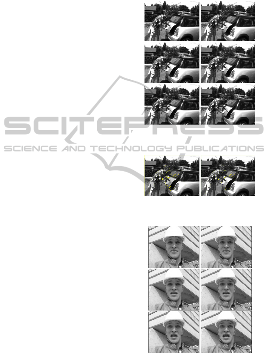
terpolation. Those are the ones that are ﬁlled-in by

inpainting. In Middlebury an intermediate frame is

given for comparison. It corresponds to the fourth im-

age in Figure 3. The RMSE is in this case 4.2440.

Figure 5 shows the interpolation between two dif-

ferent frames of the sequence Foreman. The person is

opening the mouth and some regions are disoccluded.

The maximum displacement is 9.8331. From left to

right and top to bottom, the ﬁrst and last images be-

long to the original sequence. The four intermediate

frames have been interpolated. In Figure 6 we show

the holes generated by the interpolation process. The

left image shows the holes after forward interpolation,

the right image shows the remaining ones after back-

ward interpolation which we ﬁlled-in by inpainting.

Figure 7 shows the interpolation of four frames

from a sequence where a placard is being dis-

occluded. Figure 8 shows the interpolation

of an intermediate frame in the sequence Ur-

ban taken from Middlebury. The camera moves

right and there are occlusions between buildings.

The experiments displayed here can be found in

http://www.dtic.upf.edu/∼cballester/demos/scm .

In our experiments the computation time per

frame is around: 5 sec for optical ﬂow computation,

0.55 sec for the intermediate frame interpolation and

1 min for the inpainting algorithm.

4 CONCLUSIONS

We have proposed an interpolation method to pro-

duce a sequence of plausible intermediate frames be-

tween two input images. The method is based on the

exploitation of the optical ﬂow and the handling of

occlusions by means of a time coherent video seg-

mentation which produces a set of spatio-temporal re-

gions. Occlusions and dis-occlusions are identiﬁed as

the temporal boundaries where a region ends or starts,

respectively. With this we avoid the forward propaga-

tion of occluded regions. After forward propagation

of continuing regions, holes appear and we use the

backward ﬂow to propagate information not belong-

ing to starting regions from next frame. The few re-

maining holes are ﬁlled-in by inpainting. The method

permits to avoid artifacts in occluding and disocclud-

ing regions. The method is sensitive to the quality of

the optical ﬂow and requires ﬂows of high quality.

ACKNOWLEDGEMENTS

We acknowledge partial support by MICINN project,

reference MTM2009-08171, and by GRC reference

Figure 3: Intermediate frame interpolation. The ﬁrst and

last frames are original images. The intermediate ones are

interpolated.

Figure 4: Left: The holes appearing in the ﬁrst interpolated

frame of Figure 3 after forward interpolation. Right: The

remaining holes after backward interpolation.

Figure 5: Intermediate frame interpolation. The ﬁrst and

last frames are original images. The intermediate ones are

interpolated.

FRAME INTERPOLATION WITH OCCLUSION DETECTION USING A TIME COHERENT SEGMENTATION

371

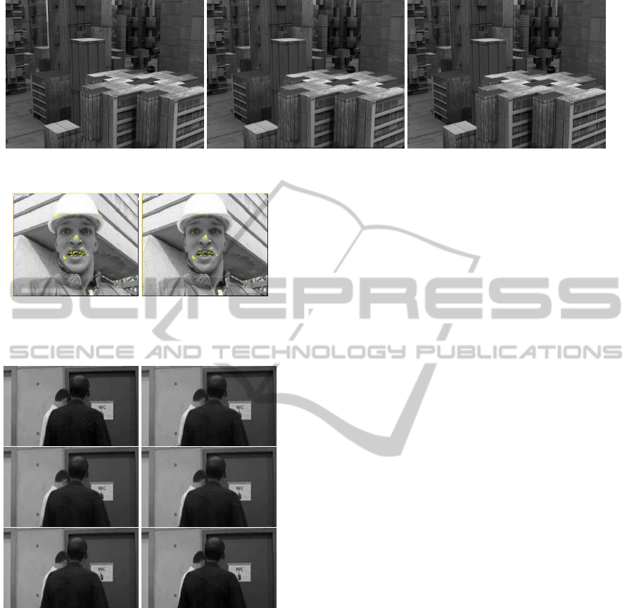
Figure 8: Intermediate frame interpolation. The ﬁrst and third frames are original images. The middle one is interpolated.

Figure 6: Left: The holes appearing in the last interpolated

frame of Figure 3 after forward interpolation. Right: The

remaining holes after backward interpolation.

Figure 7: Intermediate frame interpolation. The ﬁrst and

last frames are original images. The intermediate ones are

interpolated.

2009 SGR 773. VC also acknowledges partial sup-

port by ”ICREA Acad`emia” prize for excellence in

research funded by the Generalitat de Catalunya.

REFERENCES

Alvarez, L., Deriche, R., Papadopoulo, T., and S´anchez,

J. (2007). Symmetrical dense optical ﬂow estimation

with occlusions detection. Int. Journal of Comp. Vis.,

75:371–385.

Arias, P., Facciolo, G., Caselles, V., and Sapiro, G. (2011).

A variational framework for exemplar-based image in-

painting. Int. Journal of Comp. Vis., 93:319–347.

Baker, S., Scharstein, D., Lewis, J., Roth, S., Black, M.,

and Szeliski, R. (2011). A database and evaluation

methodology for optical ﬂow. Int. Journal of Comp.

Vis., 92:1–31.

Barnes, C., Shechtman, E., Finkelstein, A., and Goldman,

D. B. (2009). PatchMatch: a randomized correspon-

dence algorithm for structural image editing. In Proc.

of SIGGRAPH, pages 1–11.

Brox, T., Bruhn, A., Papenberg, N., and Weickert, J. (2004).

High accuracy optical ﬂow estimation based on a the-

ory for warping. In ECCV, pages 25–36.

Brox, T. and Malik, J. (2010). Large displacement optical

ﬂow: descriptor matching in variational motion esti-

mation. IEEE Transactions on PAMI, pages 500–513.

Cafforio, C., Rocca, F., and Tubaro, S. (1990). Motion com-

pensated image interpolation. IEEE Transactions on

Communications, 38:215–222.

Criminisi, A., P´erez, P., and Toyama, K. (2004). Region

ﬁlling and object removal by exemplar-based image

inpainting. IEEE Trans. on IP, 13:1200–1212.

Dane, G. and Nguyen, T. (2004). Motion vector process-

ing for frame rate up conversion. In IEEE ICASSP,

volume 3, pages 309–312.

Herbst, E., Seitz, S., and Baker, S. (2009). Occlusion

reasoning for temporal interpolation using optical

ﬂow. In Technical report UW-CSE-09-08-01. Dept.

of Comp. Sci. and Eng., University of Washington.

Ince, S. and Konrad, J. (2008). Occlusion-aware optical

ﬂow estimation. IEEE Trans. on IP, 17:1443–1451.

Koepﬂer, G., Lopez, C., and Morel, J. (1994). A mul-

tiscale algorithm for image segmentation by varia-

tional method. SIAM Journal on Numerical Analysis,

31:282–299.

Linz, C., Lipski, C., and Magnor, M. (2010). Multi-image

interpolation based on graph-cuts and symmetric op-

tical ﬂow. In 15th International Workshop on Vision,

Modeling and Visualization (VMV), pages 115–122.

Mahajan, D., Huang, F., Matusik, W., Ramamoorthi, R.,

and Belhumeur, P. (2009). Moving gradients: a path-

based method for plausible image interpolation. In

ACM SIGGRAPH, volume 28, pages 1–11.

Sun, D., Roth, S., and Black, M. (2010). Secrets of optical

ﬂow estimation and their principles. In IEEE Confer-

ence on CVPR, pages 2432–2439.

VISAPP 2012 - International Conference on Computer Vision Theory and Applications

372