GPU-FRIENDLY MULTI-VIEW STEREO FOR OUTDOOR PLANAR

SCENE RECONSTRUCTION

Hyojin Kim

, Quinn Hunter

, Mark Duchaineau

, Kenneth Joy

and Nelson Max

Department of Computer Science, University of California, Davis, CA, U.S.A.

Lawrence Livermore National Laboratory, Livermore, CA, U.S.A.

Keywords:

Multi-view Stereo, 3D Reconstruction, Planar Reconstruction, GPGPU.

Abstract:

This paper presents a new multi-view stereo approach that reconstructs aerial or outdoor scenes in both a

planar and a point representation. One of the key features is to integrate two heterogeneous schemes for planar

and non-planar reconstruction, given a color segmentation where each segment is classiﬁed as either planar

or non-planar. In planar reconstruction, an optimal plane for each segment is chosen among possible plane

candidates by comparing the remapped reference segment region with multiple target images in parallel on a

GPU. In point reconstruction for non-planar objects, remapped pixel descriptors along an epipolar line pair

are efﬁciently matched on a GPU. Our method also detects and discards incorrect segment planes and outliers

that have a large 3D discontinuity with the neighboring segment planes. Several aerial and outdoor scene

reconstruction results with quantitative analyses are provided.

1 INTRODUCTION

Traditionally, multi-view reconstruction methods be-

gin 3D scene recovery from a set of images with dense

point matching, using pixel neighborhood color simi-

larity or feature descriptors. Outliers due to matching

error are discarded or adjusted via local smoothing

or global energy minimization. A disparity map de-

rived from the set of matched pairs is converted into a

3D depth map via triangulation. Color-segmentation-

based algorithms perform a similar procedure, with

each segment reconstructed as a plane (or a smooth

surface) by least-squares or RANSAC plane ﬁtting,

given initially matched points. (Tao and Sawhney,

2000; Hong and Chen, 2004; Taguchi et al., 2008;

Bleyer et al., 2010).

In textureless regions or wide-baseline stereo,

however, plane ﬁtting may not be successful due to

numerous outliers in the initial matching. T-junctions

(i.e., incorrectly matched apparent endpoints on par-

tially occluded edges) may cause critical errors in the

plane ﬁtting. A more robust planar reconstruction is

desirable that can handle such cases. The basic as-

sumption that each segment is planar may also not be

applicable to a variety of object surfaces in outdoor

scenes. Additionally, over-segmentation, preferred in

most algorithms so that fewer segments contain re-

gions in more than one plane, may not be practical for

large planar segment regions.

In this paper, we propose a new GPU-based multi-

view stereo algorithm for aerial/outdoor urban scenes

that integrates planar and point reconstruction meth-

ods. Based on the segment properties obtained from

color segmentation, each segment is reconstructed ei-

ther as a plane or as a set of points. This method also

detects and discards incorrect segment planes and out-

liers that have a large 3D discontinuity towards neigh-

boring segment planes or points.

Our proposed algorithm is parallelized onto a

GPU where multiple GPU threads are efﬁciently uti-

lized for higher performance. In the planar recon-

struction, multiple plane-ﬁnding energy computations

are performed in parallel on a GPU to reduce compu-

tation time. In the point reconstruction, all pixels in a

descriptor form are remapped with respect to camera

geometry to improve the efﬁciency of the data access

on a GPU. We provide several aerial/outdoor urban

scene reconstruction results, with quantitative analy-

ses to evaluate the GPU speedup of our algorithm.

This paper is organized as follows: Section 2 dis-

cusses previous work, together with our contribution.

Section 3 gives an overview of the proposed algo-

rithm. Sections 4 and 5 describe the planar and point

reconstruction method, respectively. Section 6 pro-

vides experimental results with discussion, followed

by a conclusion in section 7.

255

Kim H., Hunter Q., Duchaineau M., Joy K. and Max N..

GPU-FRIENDLY MULTI-VIEW STEREO FOR OUTDOOR PLANAR SCENE RECONSTRUCTION.

DOI: 10.5220/0003825502550264

In Proceedings of the International Conference on Computer Vision Theory and Applications (VISAPP-2012), pages 255-264

ISBN: 978-989-8565-04-4

 2012 SCITEPRESS (Science and Technology Publications, Lda.)

2 RELATED WORK AND

CONTRIBUTION

Robust Planar Reconstruction. A key feature in

our work is our robust planar reconstruction method

using color segmentation. Most segmentation-based

algorithms rely on initial matched pairs in each seg-

ment, as discussed earlier. However in a scene con-

taining T-junctions or large parallax motions, the ini-

tial matched pairs may contain numerous outliers,

which can cause incorrect plane ﬁts.

Our approach is more robust and overcomes many

potential problems such as T-junctions due to a wide-

baseline, since we ﬁnd an optimal plane by directly

remapping each segment, using the homographies

from the candidate plane, onto all visible target im-

ages. One related approach is Patch-based Multi-

View Stereo (PMVS2) (Furukawa and Ponce, 2009)

that uses small patches (e.g., 5 × 5) on which to ﬁt

planes. PMVS2 also relies on initial matched pairs

(e.g., Harris corner with LoG operators) so the algo-

rithm may lead to incorrect patches. When PMVS2

fails to expand a patch’s size, holes or gaps may also

occur.

In addition, most segmentation-based stereo algo-

rithms use a disparity map between a stereo-rectiﬁed

image pair. This is not practical in multi-view cases

where we ﬁnd a plane that satisﬁes multiple images in

which the segment is visible. Moreover, in multi-view

cases with widely different camera positions and di-

rections, camera poses cannot be manipulated to pre-

vent large distortions after stereo-rectiﬁcation.

Another related approach is Iterative Plane Fit-

ting (Habbecke and Kobbelt, 2006) by computing a

plane that approximates part of the scene. However,

this method requires manual plane initialization. In

addition, since it relies on intensity differences be-

tween reference and comparison images, it may not

be sufﬁcient to ﬁnd the correct plane in wide-baseline

stereo. Our method, on the other hand, improves

planar reconstruction by exploiting several matching

constraints. The Iterative Plane Fitting method does

not detect occlusion, whereas our method simultane-

ously detects occluded planar segments in the recon-

struction process.

Plane Sweeping is another approach to reconstruct

planar scenes. Gallup et al. (Gallup et al., 2007)

proposed a real-time plane sweeping stereo method

for outdoor scenes. However, their method requires

initial sparse correspondences and uses intensity dif-

ferences only, which has limitations in wide-baseline

stereo, as mentioned earlier.

In addition, our method use a simple segment

graph to ﬁlter out plane outliers, that is, any segment

that has a large 3D discontinuity between adjacent

plane segments is ﬁltered out. Some papers such as

(Taguchi et al., 2008) use similar techniques that op-

timize segment planes. However, their optimization

again uses a simple energy function based on a dis-

parity map between a stereo image pair, which is not

applicable to multi-view cases. We believe it is more

practical and reliable to directly look at planes in 3D

instead of a disparity map in an image domain.

Hybrid Reconstruction with Segmentation. We

also seek an integration of two heterogeneous meth-

ods for aerial and outdoor urban scene reconstruction.

Our algorithm uses color segmentation to obtain seg-

mented regions to be categorized by potential 3D ge-

ometry. We deﬁne a simple planarity criterion by seg-

ment color and size so that each segment, treated as

either planar or non-planar, is reconstructed as a plane

or a set of points, respectively.

GPU-friendliness. For a CPU implementation, our

planar reconstruction could potentially be slower than

other matching approaches when a segment is too

large, since for every pixel in the segment, bilinear in-

terpolation at its reprojected target position is required

for every target view. Likewise, the descriptor com-

parison for point-to-point matches can be very expen-

sive when a scene demands many per-pixel matches.

Our algorithm is portable to GPU systems, where it

produces matches in a fraction of the time of a CPU

version, using the texture mapping hardware in the

GPU to do the bilinear interpolation for the remap-

ping.

3 RECONSTRUCTION

OVERVIEW

Our reconstruction process begins with a color seg-

mentation, in particular, mean-shift color segmenta-

tion (Comaniciu and Meer, 2002). Once segmenta-

tion is completed, any tiny segment inside a larger

segment that has a similar color is merged with

it. Sparse feature-point matching using SURF (Bay

et al., 2008), followed by triangulation, is additionally

performed to determine an approximate 3D bounding

box of the scene. This bounding box is later used to

limit the extent of plane candidates in the planar re-

construction and to ﬁlter outliers in the point recon-

struction.

During the reconstruction process, each segment

is classiﬁed as either planar or non-planar. How-

ever, it is extremely difﬁcult to automatically recog-

VISAPP 2012 - International Conference on Computer Vision Theory and Applications

256

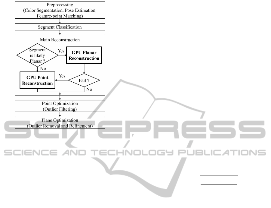
Figure 1: Reconstruction process overview.

nize whether or not a segment is planar without ex-

plicit prior knowledge. Instead, we deﬁne a simple

planarity criterion by segment size and color. For

outdoor urban scenes, most building walls and roof,

roads, and other artiﬁcial structures consist of planes,

where our planar reconstruction (Section 4) is used.

In the case of small segments (even ones as parts

of larger planes), our point reconstruction method

(Section 5) is used. Since small planar objects are

more difﬁcult to ﬁt by a plane due to higher ambi-

guity in matching projections, we treat them as a set

of points to be reconstructed. If the segment color is

close to green when examining it in both RGB and

HSV format, the point reconstruction is also used, as

this is likely a tree, bush, or similar non-planar object.

Also, the point reconstruction is applied to any seg-

ment where the planar reconstruction fails. A seman-

tic classiﬁcation approach with more intricate object

deﬁnitions could be used for a more robust classiﬁca-

tion. Figure 1 gives an overview of our reconstruction

process.

4 PLANAR RECONSTRUCTION

An initial plane for a given segment is found among

all possible planes by sampling the epipolar 3D rays

of three corners of the segment, taking all planes

through one sample on each ray, and choosing the

best. More optimal planes are then searched in a hi-

erarchical coarse-to-ﬁne manner. This whole search

narrows down the set of candidate planes for faster

computation. A later ﬁltering step gets rid of any out-

liers by checking adjacent segment planes for geomet-

ric consistency.

4.1 Model

Let I

and I

denote, respectively, the reference im-

age and i-th image in the set I of target images. For

each segment S ∈ I

, we ﬁnd an optimal plane P that

satisﬁes several constraints described below among I

and the I

∈ I in which S is visible. (Visibility is de-

scribed in the “visibility detection” section below.) In

other words, we look for a plane P that has a good in-

tensity/color matching with as many target images as

possible. These constraints are deﬁned as an energy

function to be minimized.

Color Matching. The ﬁrst constraint determines if

a plane segment is matched to other images in which

it is visible by its color (or intensity in gray-scale im-

ages). An optimal segment plane P should have a

lower color difference with its homography-projected

region in a target image. The color energy function,

based on the root mean square difference, is deﬁned

color

(P) =

∑

∈I

V (i)C

(P)

∑

∈I

V (i)N

(P)

(1)

where C

(P) is the sum of squared color differences

between reference segment S and target image I

, and

(P) is the number of pixels in the segment visible

in target image I

. V (i) determines whether or not S

is visible in target image I

, and is described later in

equation (8). C

(P) and N

(P) are deﬁned as

(P) =

∑

(x,y)∈S

∗

(x, y))M

(x, y, H

(x, y)) (2)

(P) =

∑

(x,y)∈S

∗

(x, y)) (3)

where S

∗

is the axis-aligned bounding box of the seg-

ment S and H

(x, y) is the image of (x, y) under the

homography between I

and I

. The boundary clip-

ping function W

indicates whether or not a pixel is

within target image I

, and M

measures the squared

difference between the reference color of a pixel (x, y)

and the bilinear interpolation of the target color at the

homography mapped position (x

, y

) of the pixel in a

target image I

. The deﬁnitions of W

and M

are

, y

) =



1 if (x

, y

) ∈ I

0 otherwise

(4)

(x, y, x

, y

) = |I

(x, y)− I

, y

))|

(5)

GPU-FRIENDLY MULTI-VIEW STEREO FOR OUTDOOR PLANAR SCENE RECONSTRUCTION

257

Boundary Matching. The second constraint deter-

mines if boundary pixels from the reference segment

are likely to be remapped into target boundary pixels.

We deﬁne the energy function as

bound

(P) = NN

−

∑

∈I

∑

(x,y)∈S

(x, y)) (6)

where N is the total number of target images, S

is the

set of the boundary pixels in the reference segment,

and N

is the size of S

. B

, y

) is 1 if (x

, y

) is on

or near boundary pixels (within 3 pixels in our exper-

iments) in a target image I

, and 0 otherwise.

Visibility Detection. The visibility of S under the

homography from a candidate plane P to a target

image I

is computed by checking the plane normal

(back-facing or not), the boundary clipping, and the

occlusion. We deﬁne the energy function as

visibility

(P) = N −

∑

∈I

V (i) (7)

V (i) =











0 if P is back-facing in I

0 if

(P)

∗

< δ

0 if

(P)

< γ

1 otherwise

(8)

where N

∗

is the number of pixels within the seg-

ment’s bounding box. N

indicates the number of

good matching pixels in segment S and N

is the num-

ber of pixels in S. The ﬁrst constraint determines if

this plane is back-facing or not by checking the nor-

mal and the camera direction. The second one indi-

cates how much of the mapped H

(S) is clipped away

by the boundary rectangle of image I

. In our experi-

ments, δ is approximately .5.

The third constraint measures the occlusion of

a segment by counting the number N

(P) of good

matches. A good matching pixel is a pixel that has

a small color difference (e.g., < 20 for a range of 0

to 255) between the reference segment and the target

image. If the color difference is greater, we assume

that the 3D surface point projecting to the pixel is oc-

cluded in image I

. We want to choose a plane that

generates more visible pixels, which prevents us from

choosing a slanted plane that may have a low color

difference. In our experiments, γ is approximately .7.

4.2 Initial Matching and Reﬁnement

The initial matching process is as follows. First,

three corner pixels of each segment are selected, and

their camera rays (epipolar lines) in 3D are computed.

Figure 2: Initial segment plane matching.

Each camera ray has a certain range, determined from

the precomputed 3D bounding box. Each camera

ray range is discretized into K samples and choosing

one sample on each ray results in K

possible planes.

Given each possible plane, we compute its homog-

raphy and then check the energy functions deﬁned

above by reprojecting the segment onto target views,

as shown in Figure 2.

The candidate planes are sorted by E

visibility

(P) in

equation (7). Among the planes that are visible in

the most target images, that is, that have the smallest

visibility

(P), we choose a plane that has the minimum

energy E

color

(P) in equation (1) and also has at most

twice the minimum energy E

bound

(P) in equation (6).

Once an initial plane is chosen, we again search the

camera rays in a hierarchical manner, by sampling

the rays in smaller intervals near the points deﬁning

the optimal plane P, to obtain a better plane. Such

a coarse-to-ﬁne matching increases the accuracy with

less computation time than a complete high resolution

search.

4.3 Filtering

Further steps ﬁlter out any outliers from the initial

plane matching. First, we ﬁlter out any bad plane

by examining the score from equations (1) and (7).

If the plane’s visibility energy E

visibility

(P) is close to

N, which indicates the segment is occluded in most

target views, it is removed. If the plane’s color en-

ergy E

color

(P) is more than 20, it is also ﬁltered out.

We perform another ﬁltering for the remaining planes,

using a simple segment graph where each node rep-

resents a segment and each edge represents a con-

nectivity between adjacent segments. By examining

each segment’s neighboring segments, any segment

plane that has no adjacent planes in 3D (i.e., a seg-

ment has a large 3D discontinuity with all adjacent

segments in the reference image) is also discarded.

Those discarded segments are again matched as indi-

vidual points in the following point reconstruction.

VISAPP 2012 - International Conference on Computer Vision Theory and Applications

258

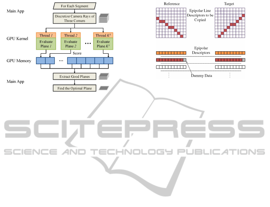
Figure 3: GPU thread utilization for plane matching.

4.4 GPU Implementation

To achieve higher performance, the energy score eval-

uation for each plane candidate is independently ex-

ecuted in parallel, as illustrated in Figure 3. In gen-

eral, the number of GPU threads is equivalent to the

number of candidate planes. Candidate planes that are

invisible in any target view, however, are discarded

prior to the GPU computation for better workload bal-

ance in all GPU threads.

Initially, all required data such as images, camera

poses and segments are copied into the GPU mem-

ory so that they can be reused during the entire plane

matching process. All input images are loaded into

a single 3D texture (but used as an array of 2D tex-

tures) to use built-in bilinear texture interpolation in

the GPU. Each thread computes energy functions for

a certain candidate plane. Then all computed results

are simultaneously written to the global memory. For

the memory access coalescing, all allocated data (e.g.,

plane coefﬁcients and energy results) in the global

memory are properly aligned.

Once all GPU threads compute the energy of all

the candidate planes, the result is copied back to the

CPU memory. We then choose several good planes

that have the minimum energy E

visibility

(P). Among

the good planes, an optimal plane is chosen by the

criterion described in the last paragraph of section 4.2.

5 POINT RECONSTRUCTION

Segments not categorized as planes are reconstructed

as a set of 3D points. The goal is to achieve an efﬁ-

cient dense reconstruction at each non-planar segment

to better represent the complex geometry of the non-

planar surface.

Unless in the form of a stereo-rectiﬁed image

Figure 4: Epipolar descriptor arrangement.

pair, dense matching tends to require lots of non-

localized data access. This is exacerbated when us-

ing multidimensional descriptors. Efﬁcient process-

ing on a GPU, with its limited memory size, demands

an efﬁcient manner of accessing pixel descriptor data

to solve as many pixels as possible using the least

amount of data. Our method seeks to leverage epipo-

lar geometry in non-rectiﬁed images to increase the

efﬁciency of the point correspondence calculation.

The point reconstruction uses dense DAISY de-

scriptors (Tola et al., 2010) to match as many pixels

as possible in non-planar segments. The DAISY de-

scriptors are formed from appending the descriptors

at a given pixel across the color channels. That is,

each pixel (x, y) stores a set of channel-appended de-

scriptor vectors D(x, y), each of which is a descriptor

vector of a given color channel:

D(x, y) = [D

(x, y) : D

(x, y)] (9)

For a more computationally efﬁcient data struc-

ture, we use the epipolar geometry to rearrange the

appended descriptors (hereafter referred to as simply

descriptors) into a linear array in the GPU memory,

which localizes data access to the descriptors.

For a given pixel p

in a reference image I

, there

is an epiolar line l

in a target image I

. Similarly, a

pixel p

along l

corresponds to an epipolar line l

reference image I

. Epipolar geometry then stipulates

that if any pixel p

on l

has a match, it must appear

in l

and vice versa. We develop the rearrangement of

descriptor data using this property.

5.1 Epipolar Data Localization

For the given reference image I

, we select a pixel

from the set U of pixels from all segments to be

reconstructed as points, and ﬁnd the epipolar line l

target image I

. We also calculate the epipolar line l

for image I

from a point on l

. We record the epipolar

line pair L = (l

, l

), and also record the pixels that l

GPU-FRIENDLY MULTI-VIEW STEREO FOR OUTDOOR PLANAR SCENE RECONSTRUCTION

259

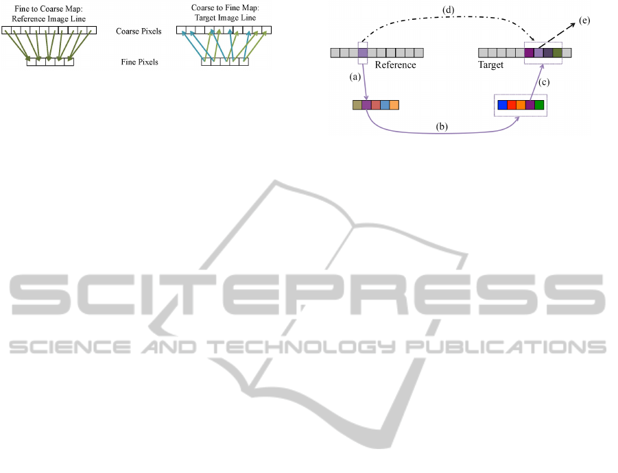
Figure 5: Coarse-to-ﬁne pixel mappings.

covers in U. This process is repeated until all pixels

in U are covered.

The epipolar line pairs are sampled such that the

number of samples remains constant. We sample

given epipolar line pair L in a fashion such that ev-

ery integer width and height in its path is covered at

least once.

This produces a line with a maximum sample

count equal to the larger of the width or the height

of the image. For lines with less than this maximum

amount of samples, their remaining points are given

dummy sample values, as shown in Figure 4.

We rearrange the DAISY descriptor data to ﬁt the

epipolar line pairs such that adjacent memory loca-

tions contain the descriptors of adjacent pixels on the

same epipolar line. We give the dummy pixels added

to maintain consistent line sizes descriptors that are

distant numerically from what a descriptor could rea-

sonably be.

5.2 Coarse-to-ﬁne Mapping

For a set of sampled epipolar lines in a given image,

we also calculate the lines as they appear in a down-

sampled version of the original image. Descriptors

created from the down-sampled version are then rear-

ranged in the epipolar fashion of the previous section.

During this process, we save a mapping of every

ﬁne-level pixel in a reference image epipolar line to

its best representative sample in the down-sampled

version for the reference image, as shown in Figure

5. For a target image, we create mappings from every

coarse-level pixel to a range of pixels on the ﬁne-level

epipolar line. This range should contain the points on

the ﬁne level that a pixel at the coarse level could map

to.

5.3 Point-to-point Matching

Once descriptors are arranged at both coarse and ﬁne

levels, we match pixels from a reference line to its

target line by minimizing the euclidean distance of the

associated descriptor vectors.

The candidate set of matched pixels at the ﬁne

level for each reference pixel is modiﬁed by the

coarse-to-ﬁne mappings. For a given reference pixel

and line pair, we ﬁrst use the ﬁne-to-coarse map-

pings and match the coarse version of the reference

Figure 6: Coarse-to-ﬁne search trajectory. (a) Map to

coarse. (b) Match coarse to coarse descriptors. (c) Fine

subset from coarse match. (d) Match ﬁne in ﬁne subset. (e)

Write out ﬁne match.

pixel to the line of coarse-level candidate pixels. The

coarse-to-ﬁne mapping of this coarse matched pixel

gives a subset of ﬁne-level candidate pixels to be

matched. Figure 6 illustrates the coarse-to-ﬁne de-

scriptor search.

After matching the pixels of a reference line l

, the

descriptor matches are translated back to the actual

image plane locations of the pixels and triangulated

to ﬁnd the 3D points. In the matching process, we

use cross-checking to get rid of outliers (e.g., occlu-

sion), that is, given a matched point in the target im-

age, we apply the matching method in reverse to ﬁnd

its matched point in the reference image. Then the

original reference point is compared with the matched

point to see if both are the same or similar within a

threshold. 3D points outside the bounding box are

also ﬁltered out.

5.4 GPU Implementation

For the GPU implementation, we load the descriptor

data at the coarse and ﬁne levels and the mappings

between them into GPU memory for a set of epipolar

line pairs. Because of each epipolar line pair has its

own data independent set of Epipolar Descriptor lines

(see Figure 4), we arrange GPU thread-blocks around

an individual pair of epipolar lines. Each thread

within one of these thread blocks attempts to solve at

least one pixel or more, depending on the maximum

number of threads allowable per thread block.

Threads in a block attempt to operate on adjacent

reference descriptors on the line and, after solving

for their pixel, refer to another descriptor in mem-

ory down the reference epipolar line to solve another

pixel if necessary. The dummy pixel descriptors are

processed exactly the same as the valid descriptors,

as the dummy descriptors are distant enough to never

be a closest match. Memory access for each thread

becomes more predictable as a result of the data and

thread arrangement.

VISAPP 2012 - International Conference on Computer Vision Theory and Applications

260

6 EXPERIMENTS AND

DISCUSSION

In this section, we evaluate the effectiveness of our

algorithm with aerial/outdoor image sets. Our appli-

cation was written in C/C++ with CUDA, OpenCL

and OpenGL. All experiments were performed on an

NVIDIA GeForce 9800 GT with 512 MB video mem-

ory, or an ATI Radeon HD 4850 with 512 MB video

memory (on Intel Core I50 2.66GHz).

Datasets. Figure 7 shows sample input images used

for our experiments. We used two sets of aerial pho-

tographs of urban scenes; Carlos (Kique) Romero’s

aerial images of Stockton, California, USA (Romero,

2009), and Brett Wayne’s aerial images of Walnut

Creek, California, USA (Wayne, 2007). We also used

three outdoor image sets that have been acquired in

our lab: coffee shack, building 1, and building 2. For

camera poses, we used Bundler (Snavely et al., 2008),

given known intrinsic camera parameters. To eval-

uate the accuracy of our planar reconstruction using

ground-truth information, we also generated two syn-

thetic scenes based on a simple OpenGL polygonal

model with slightly different textures, and then cap-

tured images from several camera views.

Reconstruction Results. Figure 8 shows how our

two reconstruction methods are integrated. The left

image is one of the reference images of the building

scene. The middle image shows a mask image for

the reference image, generated by using our classiﬁ-

cation based on the segment size and color. The white

regions are reconstructed by our planar reconstruction

whereas black regions are reconstructed by our point

reconstruction. Thus two results are effectively inte-

grated, as shown in the right image.

Figure 9 shows our reconstruction results for the

two aerial scenes and the three outdoor scenes. As

shown in the aerial scene reconstruction, our pla-

nar reconstruction recovers roads, building roofs, and

other large planes whereas our point reconstruction

recovers trees, bushes, small building walls, and other

small objects. We then render the reconstructed

point cloud using Mesh Lab (Cignoni and Ranzuglia,

2011). For the Stockton data, although most roads are

extremely large segments where many pixels in the

segments are out of image windows in target images,

many roads are reconstructed properly. The outdoor

scene reconstruction results also look quite dense. In

particular, the coffee shack and building 1 show that

our reconstruction can work properly for textureless

regions. In the coffee shack data, most of the roof and

Table 1: Accuracy of the reconstructed synthetic scenes be-

tween our planar reconstruction and PMVS2. Error indi-

cates distance between the reconstructed and the ground-

truth surface.

Error Our Method PMVS2

Synthetic

Scene 1

Min. 0.000 0.036

Max. 5.954 27.581

Mean 1.857 1.965

Synthetic

Scene 2

Min. 0.000 0.057

Max. 29.589 18.900

Mean 2.446 2.234

walls are correctly reconstructed although they con-

tain textureless regions.

Comparison with PMVS2. Figure 10 compares

our results and PMVS2 results using several scenes.

Because of the larger plane regions (one segment is

a large plane region), our result looks more dense

and detailed without many holes or gaps, compared to

the results of PMVS2, which attempts to solve small

piecewise planes with no regard to expected geome-

try. For instance, our method produces more dense re-

constructions in the synthetic scenes which contain T-

junctions with large textureless planar regions. In the

PMVS2 results, on the other hand, there are incom-

plete surface patches, probably due to mismatched

keypoints or patch extension failure.

Table 1 gives a quantitative evaluation between

our planar reconstruction and PMVS2 that measures

the accuracy of the reconstructed results of the two

synthetic scenes, compared to the ground-truth infor-

mation. Although our results look more dense than

PMVS2 result as shown in Figure 10, both results

show similar accuracy.

The separation of reconstruction methods accord-

ing to expected scene geometry frees us to use the

more distinct pixel descriptors to solve non-planar

segments such as the bushes and trees in Figure 10,

which may not be well modeled as small planes. In

general, segment categorization by predicted geome-

try prevents us from having to optimize a single re-

construction method that may not be appropriate for

all scene geometries and textures.

GPU Speedup. We also evaluated the performance

gain of our GPU-based implementation. For this anal-

ysis, we also implemented a CPU version without

parallelization. Figure 11 shows performance differ-

ences between the CPU version and our GPU version

in the planar reconstruction of the Stockton dataset.

The speedup of our GPU-based planar reconstruction

is 8.7× on average (Min.: 0.4×, Max.: 39×).

The GPU speedup of our point reconstruction is

GPU-FRIENDLY MULTI-VIEW STEREO FOR OUTDOOR PLANAR SCENE RECONSTRUCTION

261

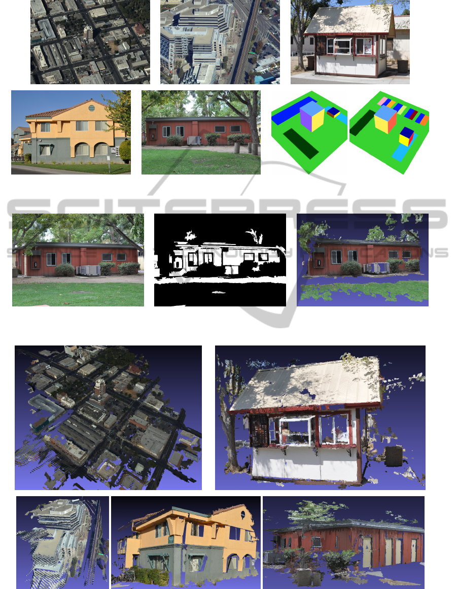
Figure 7: Input images for our experiments. From left to right and top to bottom, Stockton (CA, USA), Walnut Creek (CA,

USA), coffee shack, building 1, building 2, synthetic scene 1 and synthetic scene 2.

Figure 8: Reconstructed results integrated from our planar- and point-reconstruction methods, rendered by Mesh Lab. One of

the reference images (left), the masked image (middle), the reconstructed scene (right).

Figure 9: Reconstructed results, rendered by Mesh Lab. From left to right and top to bottom, Stockton (CA, USA) (left top),

Coffee shack (right top), Walnut Creek (CA, USA) (left bottom), building 1 (middle bottom) and building 2 (right bottom).

VISAPP 2012 - International Conference on Computer Vision Theory and Applications

262

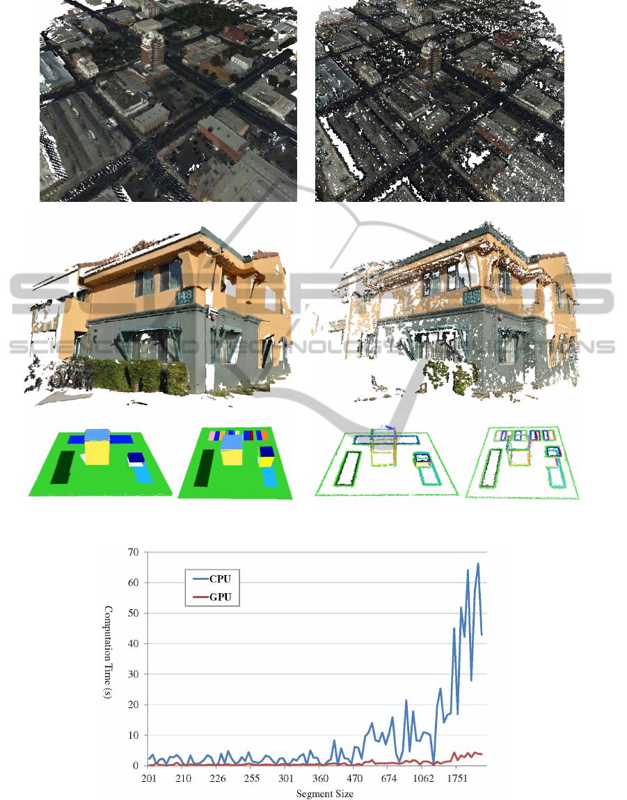
Figure 10: Comparison with PMVS2. Our reconstructed results (left column), and results from PMVS2 (right column).

Figure 11: Performance comparison between the CPU- and the GPU-version in our planar reconstruction. In the graph, the

x-axis represents segment size (# of pixels) and the y-axis represents computation time (in seconds).

GPU-FRIENDLY MULTI-VIEW STEREO FOR OUTDOOR PLANAR SCENE RECONSTRUCTION

263

Table 2: Epipolar matching execution time (in seconds) in

our point reconstruction.

Data Set CPU GPU Speedup

Stockton 5.279 0.824 6.41×

Walnut Creek 5.276 0.823 6.41×

Coffee shack 6.026 1.612 3.74×

dependent on image resolution and the maximum

threads per block, with larger resolutions requiring

each thread to solve more points. Table 2 gives aver-

age time measurements to solve 5 epipolar line pairs.

The Stockton and Walnut Creek scenes required 4

pixels to be solved per thread, while the coffee shack

scene required 8 pixels to be solved per thread.

7 CONCLUSIONS

We described a hybrid reconstruction algorithm using

GPU parallelism that reconstructs aerial or outdoor

urban scenes in a point or in a planar representation.

The reconstruction process recovers a scene that con-

tains both planar objects (e.g., building roofs, roads)

and non-planar objects (e.g., trees), classiﬁed by the

segment color and size. Our algorithm is also useful

for a scene containing large planar regions. Both re-

constructions are efﬁciently performed in parallel on

a GPU.

For future work, one can optimize the planar re-

construction using a Markov random ﬁeld with a

global energy minimization to reduce plane error be-

tween adjacent plane segments. For more robust clas-

siﬁcation between planar and non-planar objects, one

can apply a sophisticated semantic scheme by looking

up the object identiﬁcation among a large number of

training objects and/or by analyzing the texture pat-

tern.

ACKNOWLEDGEMENTS

This work was performed in part under the auspices

of the U.S. Department of Energy by Lawrence Liver-

more National Laboratory under Contract DE-AC52-

07NA27344.

REFERENCES

Bay, H., Ess, A., Tuytelaars, T., and Gool, L. V. (2008).

Surf: Speeded up robust features. In Computer Vision

and Image Understanding, volume 110, pages 346–

359.

Bleyer, M., Rother, C., and Kohli, P. (2010). Surface stereo

with soft segmentation. In IEEE Conference on Com-

puter Vision and Pattern Recognition, pages 1570–

1577.

Cignoni, P. and Ranzuglia, G. (2011). Mesh lab. Website.

available at http://meshlab.sourceforge.net.

Comaniciu, D. and Meer, P. (2002). Mean shift: A robust

approach toward feature space analysis. IEEE Trans-

actions on Pattern Analysis and Machine Intelligence,

24:603–619.

Furukawa, Y. and Ponce, J. (2009). Accurate, dense, and

robust multi-view stereopsis. IEEE Transactions on

Pattern Analysis and Machine Intelligence, 32:1362–

1376.

Gallup, D., Frahm, J.-M., Mordohai, P., Yang, Q., and

Pollefeys, M. (2007). Real-time plane-sweeping

stereo with multiple sweeping directions. In IEEE

Conference on Computer Vision and Pattern Recog-

nition, pages 1–8.

Habbecke, M. and Kobbelt, L. (2006). Iterative multi-view

plane ﬁtting. In 11th International Fall Workshop, Vi-

sion, Modeling, and Visualization, pages 73–80.

Hong, L. and Chen, G. (2004). Segment-based stereo

matching using graph cuts. In IEEE Conference on

Computer Vision and Pattern Recognition, pages 74–

81.

Romero, C. K. (2009). Aerial images of Stock-

ton, California. Website. available at http://

www.cognigraph.com/kique D80-Card1 101NIKON.

Snavely, N., Seitz, S. M., and Szeliski, R. (2008). Modeling

the world from internet photo collections. Interna-

tional Journal of Computer Vision, 80.

Taguchi, Y., Wilburn, B., and Zitnick, C. L. (2008). Stereo

reconstruction with mixed pixels using adaptive over-

segmentation. In IEEE Conference on Computer Vi-

sion and Pattern Recognition, pages 1–8.

Tao, H. and Sawhney, H. S. (2000). Global matching cri-

terion and color segmentation based stereo. In IEEE

Workshop on Applications of Computer Vision, pages

246–253.

Tola, E., Lepetit, V., and Fua, P. (2010). Daisy: An efﬁcient

dense descriptor applied to wide-baseline stereo. In

IEEE Transactions on Pattern Analysis and Machine

Intelligence, volume 32, pages 815–830.

Wayne, B. (2007). Aerial images of Walnut Creek,

California. Website. available at http://

www.cognigraph.com/walnut creek Nov 2005.

VISAPP 2012 - International Conference on Computer Vision Theory and Applications

264