MACRO-CLASS SELECTION FOR HIERARCHICAL

K-NN CLASSIFICATION OF INERTIAL SENSOR DATA

Corey McCall, Kishore Reddy and Mubarak Shah

Dept. of Electrical Engineering and Computer Science, University of Central Florida, Orlando, USA

Keywords:

Macro-class Selection, Hierarchical Classiﬁcation, Human Activity Recognition.

Abstract:

Quality classiﬁers can be difﬁcult to implement on the limited resources of an embedded system, especially

if the data contains many confusing classes. This can be overcome by using a hierarchical set of classiﬁers

in which specialized feature sets are used at each node to distinguish within the macro-classes deﬁned by the

hierarchy. This method exploits the fact that similar classes according to one feature set may be dissimilar

according to another, allowing normally confused classes to be grouped and handled separately. However,

determining these macro-classes of similarity is not straightforward when the selected feature set has yet to be

determined. In this paper, we present a new greedy forward selection algorithm to simultaneously determine

good macro-classes and the features that best distinguish them. The algorithm is tested on two human activity

recognition datasets: CMU-MMAC (29 classes), and a custom dataset collected from a commodity smart-

phone for this paper (9 classes). In both datasets, we employ statistical features obtained from on-body IMU

sensors. Classiﬁcation accuracy using the selected macro-classes was increased 69% and 12% respectively

over our non-hierarchical baselines.

1 INTRODUCTION

Inertial Measurement Units (IMUs) have become per-

vasive in smartphones and consumer electronics de-

vices, and can be employed to recognize human ac-

tivities. In this paper, we attempt to classify a large

number of confusing aerobic and cooking activities

using statistical features computed from 9 degree-of-

freedom IMUs. Most previous research in this area

has focused on processing just a small number of ei-

ther simple classes on the device itself such as in

(Ganti et al., 2010) and (Saponas et al., 2008), or more

complex classes on a dedicated server such as in (Iso

and Yamazaki, 2008) and (Miluzzo et al., 2008). Al-

though high classiﬁcation accuracy is achieved, real-

world applications would beneﬁt from the ability to

classify a large number of confusing classes using the

minimal computational resources available on the de-

vice itself. This could allow for pervasive lifestyle

monitoring of more complex scenarios such as exer-

cise patterns, cooking habits, and disease symptoms,

all of which have been shown to be recognizable us-

ing on-body IMUs in (Ermes et al., 2008), (Spriggs

et al., 2009), and (Kim et al., 2009) respectively. In

order to run these types of applications on commodity

hardware, a low-cost classiﬁcation method for a large

number of confusing classes must be developed.

We examine a hierarchical version of the low-cost

algorithm, k-Nearest Neighbor (k-NN). Because of

its simplicity, traditional k-NN does not perform well

when distinguishing between similar classes which

tend to cluster together in feature space. This can be

overcome by breaking the single k-NN classiﬁer into

a hierarchical set of simpler k-NN classiﬁers in which

specialized feature sets are used at each node to dis-

tinguish within the mutually exclusive macro-classes

deﬁned by the hierarchy. For example, the two dis-

tinct actions climbing stairs and descending stairs in a

dataset of aerobic actions may be easily distinguished

from other classes such as jumping and biking when

using a feature like mean forward acceleration. How-

ever, in the same feature space, these two actions are

easily confused with one another. If mean forward

acceleration is used to place these two actions in the

same macro class, a better feature such as mean up-

ward acceleration can be used at the second level to

distinguish between the two actions.

This hierarchical classiﬁcation process is illus-

trated in Figure 1, in which test sample X is classiﬁed

into macro-class α, β, γ, or δ using a feature set, S

determined by feature selection. X is then classiﬁed

among a smaller subset of classes using S

, S

, or

106

McCall C., Reddy K. and Shah M..

MACRO-CLASS SELECTION FOR HIERARCHICAL K-NN CLASSIFICATION OF INERTIAL SENSOR DATA.

DOI: 10.5220/0003819101060114

In Proceedings of the 2nd International Conference on Pervasive Embedded Computing and Communication Systems (PECCS-2012), pages 106-114

ISBN: 978-989-8565-00-6

 2012 SCITEPRESS (Science and Technology Publications, Lda.)

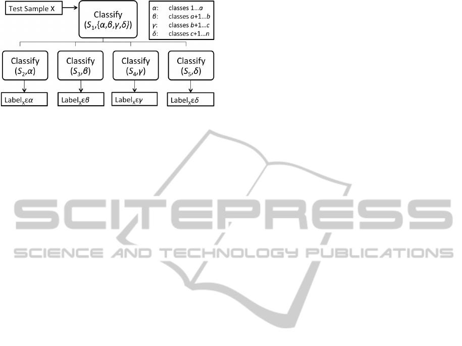
Figure 1: In this hierarchical model classiﬁer, test sample X

is classiﬁed into mutually exclusive macro-class α, β, γ, or

δ using selected feature set S

. X is then classiﬁed among a

smaller set of classes using a reselected feature set S

which

better differentiates the classes within each macro-class.

(also determined by feature selection) depending

on the macro-class. This two-tiered hierarchical de-

sign increases efﬁciency by dividing the training data

and related k-NN time complexity by the four macro-

classes, and increases classiﬁcation performance by

allowing normally confused classes to be grouped to-

gether and distinguished separately using a special-

ized set of features that differentiate them better than

the original S

. The keys to this method are: 1) ensur-

ing maximum accuracy in the top level, 2) determin-

ing appropriate macro-classes, and 3) selecting qual-

ity feature sets.

The focus of this paper is the development of

an algorithm that simultaneously determines good

macro-classes and the features that best distinguish

them, while attempting to maintain a high classiﬁca-

tion accuracy at the top level of the hierarchy. We

modify a wrapper-model greedy forward selection al-

gorithm, such that for each candidate feature set, k-

means is used to cluster the mean-centers of each

class according to the training set. A score is then de-

termined by combination of the accuracy of the clus-

tering, the number of clusters, and the evenness of the

class distribution across the clusters. As single fea-

tures are added at each iteration, the clustering accu-

racy increases while the score is maximized until an

accuracy threshold is achieved. The accuracy of the

training set is then considered adequate, and a mod-

iﬁed scoring equation is used to optimize the class

distribution while maintaining an accuracy above the

threshold. Standard greedy forward selection is then

used to select features for each classiﬁer in the second

level of the hierarchy.

The rest of this paper proceeds as follows. In Sec-

tion 2, we discuss related work on macro-class selec-

tion. In Section 3, we discuss the macro-class selec-

tion algorithm. In Section 4, we discuss the datasets

and features used to test the algorithm. In Section 5,

we compare the non-hierarchical baseline results with

those obtained with the hierarchical model. In Sec-

tion 6, we conclude the paper with a discussion of our

results.

2 RELATED WORK

The most relevant work in macro-class selection

for hierarchical classiﬁcation is given in (Wang and

Casasent, 2008). An algorithm based on “weighted

support vector k-means clustering” uses clustering to

select macro-classes to form a hierarchical classiﬁer

for multi-class classiﬁcation using a binary classiﬁer

at each node. This is similar to the one used in this

paper in that similar classes are grouped together by

clustering to build the hierarchy. However, we note

two key differences. First, this method does not in-

clude feature selection, an integral part of our moti-

vation to use multiple feature sets to improve classi-

ﬁcation performance of confusing classes. And sec-

ond, this method builds a hierarchy with an undeﬁned

number of levels based on the number of classes (each

node can handle exactly two classes/macro-classes),

whereas our method is restricted to two levels. Our

intuition is that we can minimize the misclassiﬁca-

tion of the testing data into the wrong macro-class

by limiting the number of levels in the hierarchy to

the minimum of two. Since we are attempting to im-

prove the accuracy over a non-hierarchical baseline,

any misclassiﬁcation at the top level disqualiﬁes the

test sample from being correctly classiﬁed.

In the context of feature selection using unsuper-

vised learning, (Zeng and Cheung, 2009) and (Law

et al., 2004) use feature selection with mixture model

clustering to successfully group unlabeled data. Un-

like our greedy approach, the authors’ focus on re-

moving irrelevant or redundant features at each itera-

tion of the algorithm. We choose a greedy algorithm

because of its ability to ﬁnd a smaller good solution

by starting with an empty set, reducing the complex-

ity of the resulting k-NN algorithm (perfect feature

selection is considered intractable (Kohavi and John,

1997)). Additionally, we choose a wrapper-model al-

gorithm, as opposed to ﬁlter-model, because of it’s

proven superiority in (Liu and Yu, 2005) and (Ta-

lavera, 2005). According to this research, the wrap-

per model gives better performance at the cost of a

more computationally expensive algorithm, which is

acceptable considering that the algorithm is only per-

formed in the training phase.

We also review previous work done on the CMU-

MMAC Dataset in (Spriggs et al., 2009) and (Fisher

and Reddy, 2011). Although these papers do not

use macro-classes, they provide quality baselines us-

MACRO-CLASS SELECTION FOR HIERARCHICAL K-NN CLASSIFICATION OF INERTIAL SENSOR DATA

107

ing more complex classiﬁers such as Support Vector

Machines, Hidden Markov Models, and Neural Net-

works. We discuss these results in Section 6.

Overall, the research presented in this paper ex-

tends the small amount of previous work done in

macro-class selection. The main contribution is

an algorithm that simultaneously determines quality

macro-classes and features for k-NN classiﬁcation.

The result is a set of macro-classes that can be used to

build a hierarchical k-NN classiﬁer that improves the

overall accuracy of the model when there are a large

number of confusing classes.

3 METHOD

We present our method in three parts. In Section 3.1,

we present a straightforward feature selection algo-

rithm that we use to select features for each clas-

siﬁer in the second level of the hierarchy after the

macro-classes have been determined. In Section 3.2,

we modify the algorithm for macro-class selection,

which we use to select features for the classiﬁer at the

top level of the hierarchy, as well as the macro-classes

that deﬁne the second level. In Section 3.3, we show

how both algorithms are combined to build the ﬁnal

hierarchical classiﬁer.

3.1 Base Feature Selection

Figure 2 shows a basic wrapper-model greedy for-

ward selection algorithm for feature selection. Input

to the algorithm are the training set X, consisting of M

examples, each with a pool of N scaled potential fea-

tures, and y, the corresponding label vector. The algo-

rithm keeps track of accuracy A, and a selected feature

set S. At each iteration, an exhaustive set of candidate

feature sets is built by combining the current S with

one of the potential features not in S. Each candi-

date set S ∪ {i} is then evaluated using a k-NN clas-

siﬁer with k-fold cross validation, where in this case,

k is equal to 5% of the size of the training data. In

this k-NN classiﬁer, and all subsequently referenced

in this paper, we use one nearest neighbors. If the

maximum accuracy a achieved from testing each po-

tential S ∪ {i} is less than A, S is returned as the se-

lected feature set. Otherwise, A is updated to a, and

the corresponding potential feature b is added to S.

In an attempt to further reduce the feature set and

generalize it from the training data, we eliminate all

features added to S after the ﬁnal accuracy stopped

increasing, as these features are assumed to overspec-

ify the model to the training data. For example, if the

algorithm reaches its maximum accuracy after 10 ite-

Input: X ∈ R

M×N

, y ∈ R

Output: S

[A,S] ← [0,

while |S| < N do

[a,b] ← [0,0]

for all i ∈ {1,...,N} \ S do

← KNN(X

S∪{i}

,y)

if a

> a then

[a,b] ← [a

,i]

end if

end for

if a < A then

break

end if

[A,S] ← [a,S ∪ {b}]

end while

Figure 2: We use this wrapper-model greedy forward se-

lection algorithm to select features for the classiﬁers on the

second level of the hierarchy.

rations, several unnecessary features may be added

which do not increase the accuracy, but may help ﬁnd

a better solution later on in the greedy process.

3.2 Combined Macro-class Selection

Figure 3 shows an expanded algorithm that is modi-

ﬁed to select macro-classes as it iterates. In addition

to the training data and label vector, it also requires

the target accuracy threshold t, and the total number

of classes n. The algorithm then outputs the selected

feature set as well as L, a class map that assigns each

class to one of p macro-classes, and C, the center of

each macro-class in feature space.

The algorithm starts by selecting a moderate k for

k-means clustering by taking the ﬂoor of n/

. It then

tracks the selected feature set, the accuracy, and the

corresponding outputs L and C. It then functions in

the same iterative manner with the main difference be-

ing that the performance metric is based on the quality

of the clustering at each iteration, not solely the clas-

siﬁcation accuracy as in the algorithm in Section 3.1.

The ﬁrst step in the clustering process is to calcu-

late the mean of each class in feature space (line 6 in

Figure 3). The CMEAN function simply returns this

set of points. These points are then clustered using a

modiﬁed k-means algorithm, KMEANS2. This func-

tion clusters the input into a maximum of k clusters,

where at each iteration, clusters that are empty or con-

tain less than two points are automatically dropped.

This liberal dropping scheme allows the algorithm to

determine the number of clusters in a more unsuper-

vised manner, rather than attempting to force k clus-

ters. KMEANS2 returns the cluster centers c

, the

PECCS 2012 - International Conference on Pervasive and Embedded Computing and Communication Systems

108

Input: X ∈ R

M×N

, y ∈ R

,t, n

Output: S,L,C ∈ R

p×|S|

1: k = bn/

2: [A,S,L,C] ← [0,

3: while |S| < N do

4: [a,b,ψ,l, c] ← [0, 0, 0,

5: for all i ∈ {1,...,N} \ S do

6: µ ← CMEAN(X

S∪{i}

,y)

7: {c

, p

,q} ← KMEANS2(µ,k)

8: {a

} ← KNN2(X

S∪{i}

,q)

9: if A < t then

10: ψ

← (p

> 1&@

0 ∈ l

A)?Θ(a

, p

):0

11: else

12: ψ

← (p

> 1&@

0 ∈ l

t)?Φ(a

, p

):0

13: end if

14: if ψ

> ψ then

15: [a,ψ,b,l, c] ← [a

,ψ

,i,l

]

16: end if

17: end for

18: if ψ = 0 then

19: break

20: end if

21: [A,S,L,C] ← [a,S ∪ {b},l,c]

22: end while

Figure 3: We use this modiﬁed algorithm to select features

for the classiﬁer on the top level of the hierarchy as well as

determine the macro-classes that deﬁne the second level.

number of clusters p

, and a class map q.

The accuracy of the clustering is then determined

by a modiﬁed k-NN algorithm, KNN2 (line 8). This

function ﬁrst runs a standard k-NN on X

S∪{i}

, using c

and q as a training data. KNN2 assigns each class to

a macro-class cluster based on its popularity, forming

a new class map l

. This is done instead of maintain-

ing q in an attempt to salvage good clusters that were

not evident in the mean centers, but are in the actual

training data. l

and related accuracy a

are returned.

Unlike the base algorithm in Section 3.1, our goal

is not to simply maximize the accuracy. We aim

to maximize the quality of the macro-classes while

maintaining a “good enough” accuracy. We attempt

this by building the algorithm to run in two phases.

In the ﬁrst phase (line 10), the feature with the high-

est score at each iteration is chosen as long as the

accuracy is increased, emphasizing accuracy in the

score equation Θ (Equation 1). If accuracy is not in-

creased, the feature is disqualiﬁed by setting its score

to zero. Once a certain accuracy target t is achieved,

the algorithm continues to execute in the second phase

(line 12). In this phase, the feature with the highest

score is chosen as long as the accuracy is above the

target threshold, de-emphasizing accuracy in a differ-

ent score equation Φ (Equation 2). In both phases,

clustering that results in less than two macro-classes

or empty macro-classes is automatically disqualiﬁed.

Θ =

Γ(l

)

(1)

Φ =

Γ(l

)

(2)

In the score equations, the Gamma function rep-

resents the frequency range of the class distribution

of the given class map. For example, if l

maps two

classes to macro-class α, and six classes to macro-

class β, then Γ(l

) = 6 − 2 = 4. In general, the equa-

tions guide the algorithm to choose a feature set and

macro-classes such that the accuracy and number of

macro-classes is high, and the frequency range of the

class distribution is low. In the ideal case, this should

produce a fairly even class distribution with a high

clustering accuracy of the training data.

The algorithm exits when either the current itera-

tion disqualiﬁes all candidate feature sets, or all fea-

tures have been evaluated. We note that in actual im-

plementation, we run this algorithm ﬁve times, using

the result with the highest accuracy. This is to account

for the randomness of k-means starting points. Tra-

ditionally, this is solved by using several “replicate”

starting points in the k-means algorithm itself, choos-

ing the clusters with the lowest within-cluster sums

of point-to-centroid distances. We choose to rerun the

entire algorithm because we are not necessarily inter-

ested in the best deﬁned clusters, but rather how well

they align with the training data.

3.3 Hierarchical Classiﬁcation

The process for building the hierarchical classiﬁer

from the algorithms in Figures 2 and 3 is given in the

following list.

1. Use the training data X and y, and an estimated

target accuracy t with the algorithm in Section 3.2

to select features and macro-classes for the top

level of the hierarchy.

2. Train a k-NN classiﬁer using the selected features

of X with the computed class map as the label vec-

tor, classifying the test sample into a macro-class.

3. Using the algorithm in Section 3.1, select features

for each macro-class according to the class map.

4. Train a single k-NN for each macro-class, using

only the training data corresponding to the macro-

class’s particular class set.

The process for classifying a test sample was giv-

MACRO-CLASS SELECTION FOR HIERARCHICAL K-NN CLASSIFICATION OF INERTIAL SENSOR DATA

109

en in Figure 1. Using the two-tier structure, the test

sample is processed through two k-NN classiﬁcation

algorithms, the ﬁrst to determine its macro-class, and

the second to determine its ﬁnal label.We note that al-

though the added k-NN algorithm at the top level adds

a second stage, the overall computational cost is re-

duced. This is because the k-NN algorithm at the top

level is very inexpensive considering that the train-

ing set consists of only a single point per macro-class.

At the second level, the dominating cost factor of the

algorithm (calculating the test sample’s distance from

each of the training points) is divided with the training

data between the mutually exclusive macro-classes.

4 EXPERIMENT SETUP

We test our method on human activity recognition us-

ing data collected from on-body IMU sensors. Com-

putationally inexpensive features are computed from

the data, and fed into the algorithms in Section 3 to

form the hierarchical classiﬁer. We then compare the

results to those obtained using the non-hierarchical

model built using only the base algorithm in Sec-

tion 3.1. Our goal is to show that the macro-classes

and features selected are good enough to improve the

overall performance over the non-hierarchical model.

In order for this to be achieved, there must be a

high enough performance increase by using special-

ized features on each macro-class to justify the loss in

accuracy by misclassifying data at the top level.

4.1 Datasets

We utilize two datasets: a subset of the Carnegie Mel-

lon University Multimodal Activity (CMU-MMAC)

Database (la Torre and Hodgins, 2009), and a dataset

we collected from a smartphone. In both datasets,

each IMU recorded instantaneous 3D acceleration

(accelerometer), angular velocity (gyroscope), and

orientation (magnetometer). An example of this data

is given in Figure 4. Both datasets are about the same

size, however the CMU-MMAC dataset contains

more IMUs, resulting in a larger candidate feature

pool. This is because features are computed across

each dimension of each IMU. The CMU-MMAC

dataset also contains signiﬁcantly more classes, re-

sulting in less average training data per class.

The full CMU-MMAC dataset consists of many

subjects cooking a particular recipe in an unscripted

manner while being observed by multiple sensors, in-

cluding video cameras, IMUs, motion capture, and

microphones. We use a subset of this data consist-

ing of labeled data from 5 125Hz IMUs attached to

Table 1: A list of the actions in the CMU-MMAC dataset.

1. close-fridge 16. read-box

2. crack-egg 17. spray-pam

3. open-box 18. stir-bowl

4. open-cupboard1 19. stir-egg

5. open-cupboard2 20. switch on

6. open-fridge 21. take-pan

7. pour-bowl-in-pan 22. take-egg

8. pour-bag-in-bowl 23. take-fork

9. pour-oil-in-bowl 24. take-oil

10. pour-oil-in-cup 25. take-pam

11. pour-water-in-bowl 26. twist off-cap

12. pour-water-in-cup 27. twist on-cap

13. put-pan-in-oven 28. walk–to-counter

14. put-oil-in-cupboard3 29. walk–to-fridge

15. put-pam-in-cupboard3

Table 2: A list of the actions in the smartphone dataset.

1. Biking 6. Running

2. Climbing 7. Standing

3. Descending 8. Treadmill Walking

4. Exercise Biking 9. Walking

5. Jump Roping

the subjects arms, legs, and back. The subset con-

tains 395 examples of 29 variable-length actions per-

formed by 12 subjects cooking the brownie recipe.

Labels were provided by the authors of (Taralova,

2009). The actions were chosen according to those

used in (Spriggs et al., 2009) and (Fisher and Reddy,

2011). These actions were manually segmented out of

the dataset, and all other activity was ignored. These

actions are given in Table 1. The algorithms perfor-

mance on unsegmented data is outside of the scope of

this paper, and is the focus of our future work.

The smartphone dataset was collected for this pa-

per. Each subject was given an Apple iPhone 4 loaded

with the Sensor Data application and a piece of pa-

per with the list of actions. The subject was then

instructed to start the application, perform the ac-

tion, stop the application, then write the index num-

ber next to the corresponding name on the labeling

paper. Each action was recorded 5 times by 10 sub-

jects using the single 60Hz IMU built into the phone.

This resulted in 383 total action examples (not all sub-

jects participated in each action). Once the data was

recorded, we downloaded it according to the labels

and manually trimmed each example to an 8.33 sec-

ond clip for classiﬁcation. We note that it is possible

that the task scheduler on the phone may be accessing

the sensor at a lower frequency, resulting in an incon-

sistent sample rate. The 9 actions are given in Table 2.

These datasets are ideal for testing our method,

PECCS 2012 - International Conference on Pervasive and Embedded Computing and Communication Systems

110

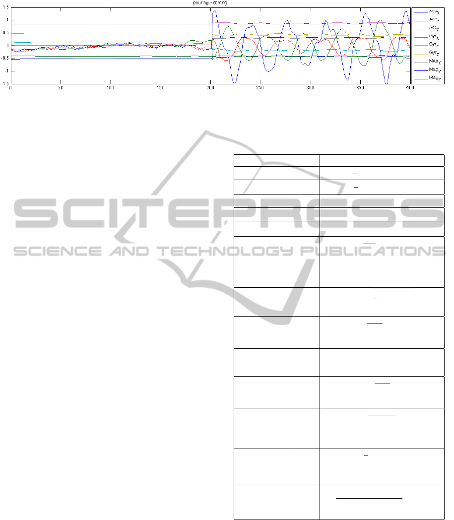
Figure 4: Each IMU in the dataset produces 9 data streams from a 3D accelerometer (Acc

X,Y,Z

), Gyroscope (Gyr

X,Y,Z

), and

Magnetometer (Mag

X,Y,Z

). This example shows the data stream from an IMU mounted on a subject’s right arm while pouring

and then stirring brownie mix. The data recorded during the transitions was removed from the dataset for our experiments.

mainly because the actions listed in Tables 1 and 2

are confusing because they are performed with sim-

ilar movement. For example, in the smartphone

dataset, the classiﬁer must distinguish walking vs.

treadmill walking as well as climbing stairs vs. de-

scending stairs and biking vs. exercise biking. The

CMU-MMAC dataset has more confusing action sets

such as walk-to-fridge vs. walk-to-counter and open-

cupboard1 vs. open-cupboard2. The CMU-MMAC

dataset also contains a larger number of classes.

4.2 Feature Calculation

We compute 13 variable-length statistical features

across the 9 dimensions of each IMU sensor. These

features, deﬁned in Table 3, form 105 potential fea-

tures for each IMU. For the CMU-MMAC dataset,

this translates to 525 features for the 5 IMUs, and for

the smartphone dataset, this translates to 105 features

for the single IMU. In each of the formulas, X

repre-

sents the ith data point of the jth dimension of the sen-

sor X (accelerometer, gyroscope, magnetometer). We

use these statistical features instead of the traditional

frequency domain or PCA features because they are

less computationally expensive to calculate, and have

been proven to be effective activity recognition de-

scriptors of IMU data in (Miluzzo et al., 2008), (Er-

mes et al., 2008), and (Karantonis et al., 2006).

4.3 Testing Procedure

We test each dataset according to the hierarchical

classiﬁcation procedure listed in Section 3.3. Leave-

one-subject-out cross validation is used in order to test

the method on each subject independently, excluding

that subject’s data from the training data used to build

the model. The results of each subject are concate-

nated to calculate the ﬁnal accuracy across the entire

dataset. The target clustering accuracy value t is se-

lected to be 90% and 95% for the CMU-MMAC and

smartphone datasets respectively. A lower target ac-

curacy is used for the CMU-MMAC dataset because

Table 3: Statistical features calculated from the IMU data.

Feature Size Formula

Mean 9 µ

∑

i=1

Variance 9 σ

∑

i=1

− µ)

Minimum 9 min

= minimum(X

)

Maximum 9 max

= maximum(X

)

Range 9 range

= max

− min

Mean

Crossing

Rate

9 mcr

`−1

∑

N−1

i=`

ϒ{(X

−

)(X

i+1

− µ

) < 0},

where ϒ is the indicator

function

Root Mean

Square

9 rms

∑

i=1

Skew 9 skew

`σ

∑

i=1

−

)

Average

Entropy

9 H

= −

∑

i=1

p(X

)

log(p(X

))

Kurtosis 9 kurt

`σ

∑

i=1

−

)

Correlation 9 corr

`σ

∑

i=1

− µ

)(X

− µ

for [a,b]={[1,2],[1,3],[2,3]}

Average

Magnitude

Area

3 SMA

∑

i=1

(|X

| + |X

Average

Energy

Expenditure

3 EE

∑

i=1

+ X

of the larger number of classes.

5 RESULTS

For each dataset, we present the total classiﬁcation

accuracy of the hierarchical model compared to the

MACRO-CLASS SELECTION FOR HIERARCHICAL K-NN CLASSIFICATION OF INERTIAL SENSOR DATA

111

non-hierarchical baseline. The top-level clustering

accuracy is also given in order to indicate how well

the macro-classes selected from the training data were

able to be generalized to the testing data, recalling that

top-level classiﬁcation accuracy signiﬁcantly impacts

performance in a hierarchical classiﬁer since it is es-

sentially the maximum achievable total accuracy.

In addition to classiﬁcation results, we also

present a novel 2D histogram matrix to show the gist

of the macro-classes selected for each dataset. The

matrices shown in Figures 6 and 7 visualize how of-

ten each class is grouped into the same macro-class

as another after the algorithm has run on all of the

subjects. Each row corresponds to a class, and the

intensity of the marking at each corresponding col-

umn represents the frequency in which the row class

was grouped into the same macro-class as the column

class. For example, the ﬁrst row in Figure 6 indicates

that action 1 is always grouped into the same macro-

class as actions 4, 6, 12, 17, 22, 23, 28, and 29 since

the marks at these columns of row 1 are completely

black. Action 5 is grouped into the same macro-class

as action 1 about 60% of the time, indicated by the

gray mark in column 5.

In addition to visualizing the gist of the selected

macro-classes, the histogram matrix can also visually

depict the quality and nature of the selected-macro

classes. The quality of the macro-class selection is

indicated by the ability of the algorithm to group the

same classes into a macro-class regardless of which

subjects the algorithm is trained on. This can be seen

in the previous example in which the column classes

with completely black marks in row 1 were always

grouped together regardless of the training set used

during cross validation. In general, we can say that a

matrix consisting of mostly black or white marks is of

good quality because the macro-classes are well de-

ﬁned across different training sets with close to 100%

or 0% matching. Additionally, if the classes are listed

in such a way that the naturally similar classes are ad-

jacent, dark clusters will form if the naturally similar

classes are generally grouped into the same macro-

class. This is further explained in Section 5.1.

In order to aid future feature selection research,

we also review which features from Table 3 were se-

lected when using each model.

5.1 CMU-MMAC Results

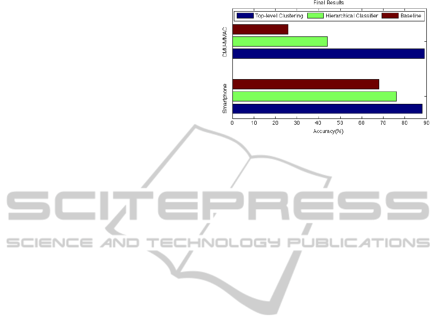
The classiﬁcation results for the CMU-MMAC

dataset are given in Figure 5. The classiﬁcation accu-

racy using the hierarchical model was 44%, a 69% im-

provement over the non-hierarchical baseline of 26%.

The top-level clustering accuracy was 89%.

Figure 5: The ﬁnal results show that the hierarchical clas-

siﬁer built using the algorithms presented in this paper out-

performs the non-hierarchical baseline in both datasets. The

high top-level clustering accuracy in both datasets indicates

the high quality of the selected macro-classes.

The histogram matrix in Figure 6 shows the gist

of the macro-class selection. Most of the graph is

completely white or very dark, indicating good qual-

ity macro-classes. In this matrix, the classes are listed

in lexicographical order, making naturally similar ac-

tions beginning with the same verb (e.g. pour-oil-in-

bowl, pour-water-in-bowl) adjacent to one another. In

this way, it can be seen that some of the macro-classes

correspond to naturally similar classes. Speciﬁcally,

the pouring actions in rows 7-11 are always grouped

together with the other pouring actions in columns

7-11, the stirring actions in columns 18-19, and the

twisting actions in columns 26-27. Theses groups are

emphasized by colored ellipses in Figure 6. The aver-

age number of macro-classes created from the 29 base

classes was 4.

5.2 Smartphone Results

The classiﬁcation results for the smartphone dataset

are also given in Figure 5. The total classiﬁcation

accuracy using the hierarchical model was 76%, a

12% improvement over the non-hierarchical baseline

of 68%. The top-level clustering accuracy was 88%.

The histogram matrix for the smartphone dataset

is given in Figure 7. Like the CMU-MMAC dataset,

most of the marks on the graph are completely white

or very dark, indicating good, subject-independent

macro-classes. We can also see that the intersec-

tions of naturally similar classes such as climb-

ing/descending and running/walking are ﬁlled with

completely black marks, indicating that these classes

were grouped together every time. The average num-

ber of macro-classes created from the 9 base classes

was 2.6.

PECCS 2012 - International Conference on Pervasive and Embedded Computing and Communication Systems

112

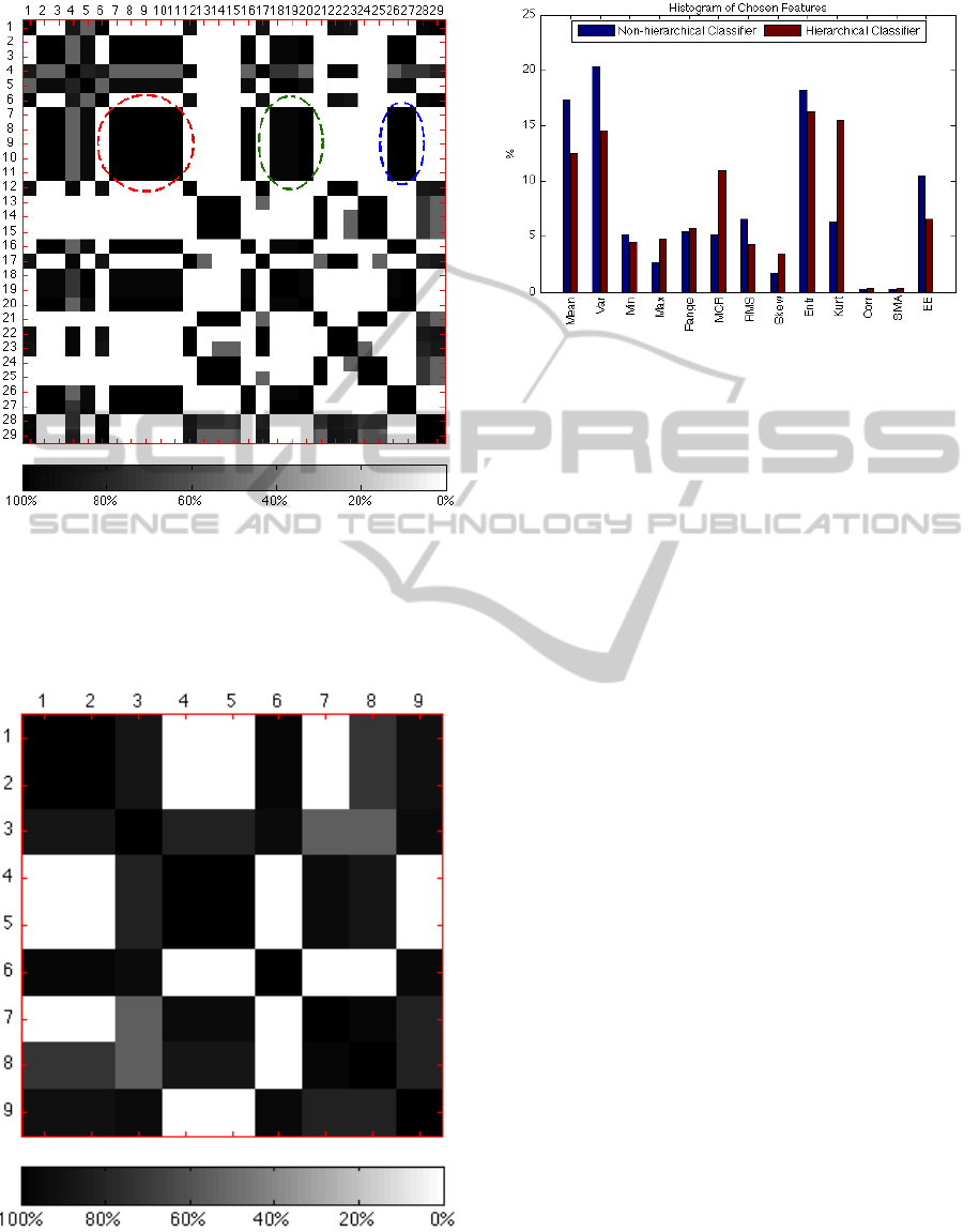
Figure 6: The histogram matrix for the CMU-MMAC

dataset. The red, green, and blue ellipses highlight how the

pouring actions are generally grouped with the other pour-

ing actions, the stirring actions, and the twisting actions re-

spectively. The index numbers correspond to the actions

listed in Table 1.

Figure 7: The histogram matrix for the smartphone dataset.

The index numbers correspond to the actions listed in Ta-

ble 2.

Figure 8: Histogram showing the distribution of the selected

features across both datasets for the non-hierarchical and

hierarchical models. The bottom labels correspond to the

features listed in Table 3.

5.3 Feature Selection Results

The distribution of the features selected is given in

Figure 8. In general, the overall most useful features

were mean, variance, and entropy, having the highest

distribution in both models. The least useful features

were the correlation and signal magnitude area, hav-

ing the lowest distribution in both models. We also

note that the standard deviation of the distribution of

the hierarchical model is 5.6, which is less than the 6.8

of the non-hierarchical model. This implies that the

features were more evenly distributed in the hierarchi-

cal model. This is expected considering that features

that are less descriptive overall are eliminated in fea-

ture selection for the non-hierarchical model, but can

be used as specialized features in one of the hierarchi-

cal model’s subclassiﬁers. This is speciﬁcally evident

in the mean crossing rate and kurtosis features, both

of which more than doubled their representation in the

hierarchical model.

6 CONCLUSIONS

The results show that our algorithm performs well

in selecting macro-classes and features for hierarchi-

cal classiﬁcation, as accuracy was improved in both

datasets over the non-hierarchical baseline. We note

that with the exception of one subject, the hierar-

chical classiﬁer either matches or outperforms the

non-hierarchical baseline for every individual subject.

This empirically shows that the macro-classes and

features selected by our algorithm are useful in cre-

ating the hierarchical k-NN classiﬁer. We emphasize

that the improvement was much greater in the more

MACRO-CLASS SELECTION FOR HIERARCHICAL K-NN CLASSIFICATION OF INERTIAL SENSOR DATA

113

complex CMU-MMAC dataset (69% vs. 12%). This

is because the hierarchical classiﬁer was built to group

and handle similar classes separately with specialized

features. Therefore, the more confusing dataset yields

a higher improvement.

However, we do recognize that although we out-

perform the non-hierarchical baselines, the resulting

accuracies are still low compared to previous work in

(Fisher and Reddy, 2011). This is because, instead of

focusing on the maximization of total accuracy as in

previous work, we focus on generating quality macro-

classes and testing the performance impact of using

the respective specialized feature sets. In an effort

to minimize the computational cost of our resulting

algorithm, we use computationally inexpensive sta-

tistical features and k-NN classiﬁcation on the sec-

ond level of the hierarchy. Our accuracy would most

likely be substantially improved at the cost of com-

putational resources by using the more complex fea-

tures and classiﬁcation methods of previous work on

the second level of the hierarchy. Once the test sample

has been correctly classiﬁed into a macro-class at the

top level (which we achieve very high performance),

we note that any type of feature set or classiﬁer can

be used by the subsequent classiﬁcation nodes.

Overall, we contribute a new algorithm to improve

the performance of the k-NN classiﬁer by building a

hierarchical classiﬁcation model with specialized fea-

ture selection. Our results show signiﬁcant improve-

ment over the baseline, with the possibility to improve

further by using more complex features or classiﬁers

on the bottom level of the hierarchy.

ACKNOWLEDGEMENTS

Data used in this paper was obtained from

kitchen.cs.cmu.edu and the data collection was

funded in part by the National Science Foundation un-

der Grant No. EEEC-0540865.

REFERENCES

Ermes, M., Parkk, J., Mantyjarvi, J., and Korhonen, I.

(2008). Detection of daily activities and sports with

wearable sensors in controlled and uncontrolled con-

ditions. IEEE Transactions on Information Technol-

ogy in Biomedicine, 12(1).

Fisher, R. and Reddy, P. (2011). Supervised multi-modal

action classiﬁcation. Technical report, Carnegie Mel-

lon University.

Ganti, R., Srinivasan, S., and Gacic, A. (2010). Multisensor

fusion in smartphones for lifestyle monitoring. In Pro-

ceedings of 2010 International Conference on Body

Sensor Networks.

Iso, T. and Yamazaki, K. (2008). Gait analyzer based on

a cell phone with a single three-axis accelerometer.

In Proceedings of 6th ACM Conference on Embedded

Networked Sensor Systems.

Karantonis, D., Narayanan, M., Mathie, M., Lovell, N., and

Celler, B. (2006). Implementation of a real-time hu-

man movement classiﬁer using a triaxial accelerome-

ter for ambulatory monitoring. IEEE Transactions on

Information Technology in Biomedicine, 10(1).

Kim, K.-J., Hassan, M. M., Na, S., and Huh, E.-N. (2009).

Dementia wandering detection and activity recogni-

tion algorithm using tri-axial accelerometer sensors.

In Proceedings of the 4th International Conference on

Ubiquitous Information Technologies & Applications.

Kohavi, R. and John, G. H. (1997). Wrappers for feature

subset selection. Artiﬁcial Intelligence, 97(1-2).

la Torre, F. D. and Hodgins, J. (2009). Guide to the

carnegie mellon university multimodal activity (cmu-

mmac) database. Technical Report CMU-RI-TR-08-

2, Carnegie Mellon University.

Law, M., Figueiredo, M., and Jain, A. (2004). Simultaneous

feature selection and clustering using mixture models.

IEEE Transactions on Pattern Analysis and Machine

Intelligence, 26(9).

Liu, H. and Yu, L. (2005). Toward integrating feature selec-

tion algorithms for classiﬁcation and clustering. IEEE

Transactions on Knowledge and Data Engineering,

17(4).

Miluzzo, E., Lane, N., Fodor, K., Peterson, R., Lu, H., Mu-

solesi, M., Eisenman, S., Zheng, X., and Campbell,

A. (2008). Sensing meets mobile social networks: The

design, implementation and evaluation of the cenceme

application. In Proceedings of 6th ACM Conference

on Embedded Networked Sensor Systems.

Saponas, T. S., Lester, J., Froehlich, J., Fogarty, J., and Lan-

day, J. (2008). ilearn on the iphone: Real-time human

activity classiﬁcation on commodity mobile phones.

Cse technical report, University of Washington.

Spriggs, E., la Torre Frade, F. D., and Hebert, M.

(2009). Temporal segmentation and activity classiﬁ-

cation from ﬁrst-person sensing. In Proceedings of

IEEE Workshop on Egocentric Vision at Conference

on Computer Vision and Pattern Recognition.

Talavera, L. (2005). An evaluation of ﬁlter and wrapper

methods for feature selection in categorical clustering.

In Proceedings of 6th International Symposium on In-

telligent Data Analysis.

Taralova, E. (2009). Cmu multi-modal activity dataset an-

notations. In http://www.cs.cmu.edu/ espriggs/cmu-

mmac/annotations/.

Wang, Y.-C. F. and Casasent, D. (2008). New sup-

port vector-based design method for binary hierarchi-

cal classiﬁers for multi-class classiﬁcation problems.

Neural Networks, 21(2-3).

Zeng, H. and Cheung, Y.-M. (2009). A new feature selec-

tion method for gaussian mixture clustering. Pattern

Recognition, 42(2).

PECCS 2012 - International Conference on Pervasive and Embedded Computing and Communication Systems

114