MONOCULAR DEPTH-BASED BACKGROUND ESTIMATION

Diego Cheda, Daniel Ponsa and Antonio M. L

opez

Computer Vision Center, Universitat Aut

onoma de Barcelona, Bellatera, Spain

Keywords:

Background Estimation, Depth Estimation, Energy Minimization, Graph Cuts.

Abstract:

In this paper, we address the problem of reconstructing the background of a scene from a video sequence with

occluding objects. The images are taken by hand-held cameras. Our method composes the background by

selecting the appropriate pixels from previously aligned input images. To do that, we minimize a cost function

that penalizes the deviations from the following assumptions: background represents objects whose distance

to the camera is maximal, and background objects are stationary. Distance information is roughly obtained by

a supervised learning approach that allows us to distinguish between close and distant image regions. Moving

foreground objects are ﬁltered out by using stationariness and motion boundary constancy measurements. The

cost function is minimized by a graph cuts method. We demonstrate the applicability of our approach to

recover an occlusion-free background in a set of sequences.

1 INTRODUCTION

During the last decade, the number of cameras has

increased dramatically. This growth has been ex-

perienced in all areas, including traditionally ones

such as video surveillance, video and photography for

professionals and enthusiasts, and systems for driv-

ing assistance, but also in newest ones like in smart-

phones, and video gaming. This growing interest was

mainly motivated by reductions in cost and improve-

ment in the quality of digital cameras. Furthermore,

the widespread use of computers has provided user-

friendly ways to process images. Even applications

for domestic use allow to any user manipulating an

image to enhance it in many forms. For instance,

image editing software includes basic tools like ad-

justing colors and cropping images, but also more

complex ones like removing disturbing elements and

merging images to compose collages or panoramas.

In this paper, we focus on how to automatically

removal transient and moving objects from a set of

images or a sequence where the background is par-

tially occluded and located at far distance from the

camera. Besides the obvious uses of this for image en-

hancement (e.g., removing objects that spoil a beau-

tiful landscape photograph, or creating images with-

out cluttered foreground objects), it has found many

other applications in computer vision and graphics

ﬁelds. For example, background estimation is usually

the ﬁrst step in background subtraction algorithms

(Radke et al., 2005), where moving objects are de-

tected by subtracting the observed image from an es-

timated reference background image. Segmentation

of moving objects provides useful information from

video processing applications such as image stitching,

background substitution, compression, and tracking.

We assume that the background is composed by

pixels representing objects whose distance to the cam-

era is maximal, as in (Granados et al., 2008). This

deﬁnition implies the knowledge of depth informa-

tion, which is commonly unavailable. However, hu-

man beings easily identify which objects are in the

foreground as well as those belonging to the back-

ground. This is because people can infer depth in-

formation even from a single image by combining

monocular cues (e.g., perspective, textures, occlu-

sions, etc.) that the visual system uses to understand

their surroundings (Goldstein, 2010). In computer

vision, estimating depths has been traditionally ad-

dressed by techniques that require multiple images

(e.g., depth from stereo). Recently, proposals on ac-

curate depth map estimations from a single image

have been done (Saxena et al., 2009). However, for

the purposes of background estimation, just a rough

distinction between close and distant image regions

can be enough. We propose a method to perform such

distinction based on a supervised learning approach.

This information is integrated in the background esti-

mation process.

Our background model is then based on two

assumptions: First, background represents objects

placed at far distances from the camera; and second,

323

Cheda D., Ponsa D. and M. López A..

MONOCULAR DEPTH-BASED BACKGROUND ESTIMATION.

DOI: 10.5220/0003816503230328

In Proceedings of the International Conference on Computer Vision Theory and Applications (VISAPP-2012), pages 323-328

ISBN: 978-989-8565-03-7

 2012 SCITEPRESS (Science and Technology Publications, Lda.)

background objects are stationary. According to that,

we deﬁne a method to select from a set of images the

appropriate pixels to compose the background. It is

based on minimizing a cost function that penalizes

deviations from our model. This method requires a

set of aligned images, and to do this accurately, we

propose an image registration process that takes ad-

vantage of our distant region segmentation method.

The rest of the paper is organized as follows. In

Sec. 2, we introduce several related works. Our

method is proposed in Sec. 3. Sec. 4 shows the ex-

perimental results. Finally, we conclude in Sec. 5.

2 RELATED WORK

Background estimation from a set of images has been

widely studied in many areas of computer vision. In

general, most of techniques to background estimation

are based on strategies to avoid the use of depth be-

cause it is commonly unavailable (e.g., Kalman ﬁl-

tering, mixtures of Gaussians, among others). In

(Harville et al., 2001), the authors exploit depth in-

formation recovered from stereo cameras to remove

the background. However, the use of stereo cameras

is often an unusual conﬁguration in most systems.

Our approach is related to those algorithms based

on energy minimization. Here, we review some of

them, and state the novelty of our proposal. Following

this strategy, in (Agarwala et al., 2004), background is

estimated from a set of images by minimizing a cost

function that penalizes the least common pixels.

In (Cohen, 2005), background estimation is for-

mulated as a labeling problem, where a cost function

penalizing stationariness and motion boundary incon-

sistencies is minimized by graph cuts.

In (Granados et al., 2008), the authors propose

a method for a set of images taken from the same

viewpoint with no restrictions on the time interval be-

tween them (i.e., non-time sequences). To do that,

they adapt the motion boundary penalty from (Cohen,

2005) to a term that does not require temporal coher-

ence.

Recently, in (Chen et al., 2010), the background is

initialized from stable areas and an image inpainting

technique is applied to predict the value of unstable

pixels. Then, higher costs are assigned to labels that

are more different from the predicted result.

Motivated by the previous works, we also consider

the background estimation as a labeling problem. We

use a similar cost function as in (Cohen, 2005), ap-

plying graph cuts to minimize it. However, to the best

of our knowledge, any previous work has taken into

account that depth information can be extracted from

single images. Then, we propose a simple method to

identify close/distant image regions and use this infor-

mation to penalize deviations from our background

model. Additionally, if there is camera motion, all

previously reviewed methods require an initial image

alignment before applying the proposed solution. We

solve this problem by aligning the backgrounds of the

input images basing on our distant region segmenta-

tion.

3 PROPOSED METHOD

3.1 Problem Statement

The input of our method is a sequence of aligned

images of a scene. Our objective is to estimate the

background by ﬁnding, for each pixel, an input image

in which the background is visible. Then, the scene

background is reconstructed by copying pixels from

the appropriate input image. Each pixel has assigned

a labeling corresponding to a frame number, and each

possible labeling has an associated cost. The goal is

obtaining a labeling that minimizes that cost.

Formally, let I = {I

, . . . .I

} be a set of N input

images. P denotes the set of pixels in an image. I

(p)

denotes the color value at pixel position p ∈ P for n-

th image I

. Let L = {1, . . . , N} be a set of labels,

each one corresponding to an image in I . A labeling

is a mapping f : P → L, that means that a pixel p ∈ P

has assigned the label f

∈ L. Each labeling f gener-

ates an image I

: p → I

(p). Then, the background

estimation problem is posed as ﬁnding a labeling f

∗

to construct the background I

= I

∗

such that f

∗

is a

minimum cost labeling. In the next sections, we for-

malize the cost function to be minimized.

3.2 Energy Function

The energy function E( f ) of a labeling f is deﬁned as

(Boykov et al., 2001)

E( f ) =

∑

p∈P

( f

) +

∑

p,q∈N

p,q

( f

, f

) , (1)

where D is the data term, and V is the smoothness

term. The data term deﬁnes the cost of assigning the

label f

to pixel p. The smoothness term is the cost

of assigning labels f

and f

to neighboring pixels p

and q, such that p, q ∈ N , being N the set of adjacent

pixels in P.

A labeling that minimize the energy E is found

by using the α-expansion algorithm implemented by

(Delong et al., 2011). For details about the optimiza-

tion algorithm, please refer to (Boykov et al., 2001).

VISAPP 2012 - International Conference on Computer Vision Theory and Applications

324

Smoothness term penalizes the intensity differ-

ences between neighboring regions (Kwatra et al.,

2003), giving a higher cost when f

and f

do not

match well

p,q

( f

, f

(kI

(p)−I

(p)k+kI

(q)−I

(q)k)

(2)

The data term penalizes the labelings that do not

hold the background model. Then, our data term ac-

counts the color stationariness D

, motion boundary

consistency D

, and proximity/distantness informa-

tion D

( f

) = αD

( f

) + βD

( f

) + γD

. (3)

Since, the three components have different units,

we ﬁrst normalize each one between 0 and 1, and then

we introduce different weights for each component to

balance the contribution of each one. The ﬁrst two

terms in D were introduced by (Cohen, 2005), and

the last term corresponds to our approach. In the next

sections, we detail each term.

3.3 Stationariness

This term penalizes image regions whose color varies

signiﬁcantly along time. The stationariness cost

( f

) assigns a high cost to pixels with large color

variance in a small time interval (Cohen, 2005). For-

mally,

( f

)=min{Var

−1, f

(p), Var

, f

(p)} , (4)

where Var

i, j

(p) is the mean of the variance of each

color channel from image I

to I

at pixel p, and f

r ∈ L denotes the r-th image posterior or previous to

the current one, respectively.

3.4 Motion Boundary Consistency

We use motion boundaries to penalize pixels corre-

sponding to moving objects. Motion boundaries oc-

cur in adjacent image regions having different image

velocities due to motion parallax or independent mov-

ing objects (Black and Fleet, 2000). Based on that,

the motion boundaries can be approximated as the

gradient of the difference between an image and the

background, which is justiﬁed since the boundary of

a moving objects occur at locations where the images

start to differ. Assuming that I

is the background

image and I

is an input image containing moving

objects, the difference image F

=k I

− I

k has

a large gradient magnitude k 5F

k where I

and

are poorly matched. Likewise, k 5I

k has large

values at intensity edges. Motion boundary consis-

tency penalizes motion boundaries that do not occur

at background’s intensity edges (Cohen, 2005)

( f

) =

∑

i∈L

k 5F

(p) k

k 5I

(p) k

+ε

, (5)

where ε is a small value to avoid zero-division.

3.5 Proximity/Distantness Information

This term penalizes those image regions which are

close in the scene, since we assume that the back-

ground is composed by distant regions. This implies

that we require at least rough information about scene

depths.

Even though depth estimation has been focused

from techniques requiring multiple images (e.g.,

depth from stereo, structure from motion, etc.), re-

cently, some proposals on depth estimation from a

single image have been done (Saxena et al., 2009).

They try to derivate exact distances to elements in

the scene. However, according to our background

deﬁnition, just having information about the proxim-

ity/distantness can be enough for background estima-

tion. Instead of estimating a continuous depth map,

we segment the distance space into close/distant re-

gions.

For computing such segmentation, we train an

AdaBoost classiﬁer based on a set of discrimina-

tive features to distinguish between both kinds of re-

gions according to a distance threshold. We use the

following features: RGB and HSV color mean and

histograms for each channel to distinguish between

different objects; texture gradients characterized by

Weibull parameters (Nedovic et al., 2010) and Ga-

bor ﬁlters to capture surface orientations; and, pixel

location to distinguish different regions in the image

(sky, ground, etc.). Our visual features are computed

at region rather than pixel level. Each image is over-

segmented into superpixels, trying approximately to

ﬁt each image region to scene objects, and each su-

perpixel is described using our visual features.

To train our classiﬁer, we use images from the

dataset provided by (Saxena et al., 2009). This dataset

has a depth map associated to each image, which is

used to label a set of positive/negative examples.

We have established the threshold to distinguish

what is a distant region at 30 m since, for the cam-

era used, beyond that distance the moving objects in

the scene just show a scarce motion in the image, and

most of them can be considered as part of the back-

ground.

Given a new image, the close/distant segmentation

is obtained from the classiﬁer predictions for each re-

gion. Results of this process are shown in Fig. 1.

MONOCULAR DEPTH-BASED BACKGROUND ESTIMATION

325

(a) Original images

(b) Distant regions segmentation

Figure 1: Results of our approach to identify close and

distant image regions: (a) Original images, (b) Computed

mask where distant regions are in red and close regions are

in blue. The ﬁrst three images are from Saxena et al. testing

set, and the last two are from video sequences.

We assign a cost to each pixel belonging to a close

region R

, which is the Euclidean distance between

that pixel and the nearest pixel belonging to a distant

region R



0 if p ∈ R

min{d(p, q) | q∈ R

} if p ∈ R

, (6)

where R

is the set of pixels belonging to close re-

gions, R

is the set of pixels in distant regions, and

d(p, q) is the Euclidean distance between two pixels

coordinates.

Basically, we are stating that a close region has

a higher associated cost when it is further away from

any distant region. We also penalize those regions that

being distant in the previous frame become closer in

the current frame, because they probably belong to

moving objects approaching to the camera.

3.6 Image Registration

The described cost minimization process can be ap-

plied as long as the set of images have been acquired

from an static camera. If the camera is not static, ﬁrst

images have to be registered. To do that, we align

each two consecutive images by using Lucas-Kanade

algorithm. To perform such alignment between the

current image I

and next image I

, we use as tem-

plate T the distant regions of I

. Distant regions

are used to align images since they behave as an in-

ﬁnity plane providing accurate information about the

camera motion, leading the images aligned with re-

spect to the background. This plays a signiﬁcant role

during penalties computation because a precise align-

ment reduces the probability of selecting wrong pixels

values to compose the background. Lucas-Kanade al-

gorithm iteratively minimizes the difference between

T and I

under the following goal objective

∑



(W (q, a)) − T (q)



, (7)

with respect to a = {a

}

i=1...6

, where W (q, a) is an

afﬁne warp

W (q, a) =



(1 + a



4 EXPERIMENTAL RESULTS

For evaluating our method we use the sequences

shown in Figs. 3-5. Figures 3 and 4 were taken us-

ing hand held consumer cameras, requiring alignment

between frames. Both sequences were extracted from

Youtube, having low-quality due to the compression

applied. However, our method shows good results

in obtaining background even under this quality. Se-

quence in Fig. 5 was taken ﬁxing the camera with

a tripod, without temporal coherence between frames

(Granados et al., 2008).

The parameters values to control the effect of each

term in the data term were experimentally deﬁned as

α=.3, β=.4, and γ=.3, which gave us good results.

The effect of each term in the energy function is

depicted in Fig. 2. First, terms are considered in

isolation (see Fig. 2(b)-(d)). All of them contribute

to reduce the transient objects. As Fig. 2(d) shows,

the proximity/distantness term in isolation keeps the

car which is located further away from the camera.

This occurs since we are not considering color or mo-

tion changes. Thus, the far-away car has a low-cost

due to it has a high probability of belonging to the

background. Then, a progressive improvement of the

background estimation is obtained by combinations

between the data term components (see Fig. 2(e)-(g)).

Finally, using all terms a signiﬁcantly improvement

is reached (see Fig. 2(h)), which implies that they

are complementary. Note also that the result of our

method overcomes the Cohen’s method result shown

in Fig. 2(e), which fails to remove some artifacts.

We compare our proposal against the popular me-

dian ﬁltering algorithm and the approach of (Agar-

wala et al., 2004), which is in the state-of-the-art of

background estimation. Figures 3-5 show the results

of applying our approach to different sequences.

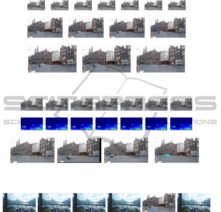
In Fig. 3, we show the result of our method in a

scene with an independent moving object (i.e., the car

approaching to the camera). Fig. 3(b) depicts how

the car is penalized since it is moving, and how the

penalization increases as the car become closer. Note

that distant regions have a low-cost due to our depth-

based term. Our method effectively removes the car

while median ﬁlter method keeps some ghost of it, as

Fig. 3(c) shows. Fig. 3(d) shows the result of Agar-

wala et al. In many cases, as in Fig. 3(f), this method

requires a user interaction to remove some artifacts

VISAPP 2012 - International Conference on Computer Vision Theory and Applications

326

(a) Original images

(b) D

+V (c) D

+V (d) D

+V (e) D

+ D

(f) D

+ D

+V (g) D

+ D

+V (h) D

+ D

Figure 2: (a) City sequence, (b)-(h) Interaction between terms. Including our term on the cost function allow us to reach a

better background estimation results. This implies that all terms are complementary.

(a) Original images

(b) Data term for images

Figure 3: (a) Seven images of the City sequence, (b) Data term for each image (red corresponds to high-cost values, blue

to low-cost values). Estimations using: (c) Our method, (d) Median ﬁlter, and (e) Agarwala et al., 2004, (f) Interactive step

required to remove some artifacts in Agarwala et al. method.

(a) Original images (b) Our method (c) Median ﬁlter (d) Agarwala et al.

Figure 4: (a) The Train sequence. Estimations using: (b) Our method, (c) Median ﬁlter, and (d) Agarwala et al., 2004.

that are still present in the obtained result. After that

step, Agarwala et al. method reaches a comparable

performance with respect to our method. In the rest

of experiments, such manual processing is performed

when it is necessary to ensure a comparable result.

Figure 4 shows an experiment done to evaluate

our method under low-quality images. This kind of

videos are not intentionally captured for extracting

the background, however it can be obtained without

transient objects. Even under low-quality videos our

proposal correctly estimates the background.

Figure 5 shows the performance our method in

a scene without temporal coherence between frames.

However, our approach behaves reasonably well un-

der this setting. Although some ghosts are present

in shadows, our results are comparable with respect

to Agarwala et al. The remaining artifacts can be re-

moved by using a gradient-domain fusion as in (Agar-

wala et al., 2004; Granados et al., 2008).

From a quantitative viewpoint, we compute the

mean absolute difference between our results against

the manually reﬁned results of Agarwala et al. The

mean of such difference is equal to 0.06, implying that

both methods are close one to another.

Despite that both methods seem to behave sim-

ilarly, our approach is fully automatic while the

MONOCULAR DEPTH-BASED BACKGROUND ESTIMATION

327

(a) Original images

(b) Our method (c) Agarwala et al.

Figure 5: (a) Images of the Market scene. Estimations us-

ing: (b) Our method, (c) Agarwala et al., 2004.

method of Agarwala et al. requires user interactions

for reﬁnement. For instance, when the estimated

background is still containing foreground objects, the

user must selects these regions which will be replaced

by new ones offered by the system. In some cases,

this interactive step must be repeatedly performed to

achieve an acceptable result. Moreover, Agarwala et

al. apply additional steps as, for instance, gradient-

domain fusion to remove image artifacts. By contrast,

our method is simpler and straightforward.

5 CONCLUSIONS

In this paper, we presented a method to back-

ground estimation containing moving/transient ob-

jects, which uses depth information for such purpose.

Usually, this information is unavailable for monocular

cameras. However, we recovered information about

proximity/distantness of a region in an image, which

is enough for our purpose. This segmentation is used

to found the background by penalizing close regions

in a cost function, which integrates color, motion, and

depth terms. We minimized the cost function by using

a graph cuts approach.

We tested our approach with sequences taken un-

der different conditions (e.g., moving/static camera,

temporal/non-temporal coherence, low/high-quality).

Experimental results shown that our method signiﬁ-

cantly outperforms the median ﬁlter approach. Also,

our approach is comparable to state-of-the-art meth-

ods. Unlike Agarwala et al., we perform this task au-

tomatically, without any user intervention.

As further work, we plan to complement our

approach with a gradient-domain fusion to remove

artifacts that are still present in dissimilar images.

Finally, we plan to focus on selecting appropriate

frames to compose the background since many frames

in a sequence do not contribute to the ﬁnal estimation.

ACKNOWLEDGEMENTS

This work is supported by Spanish MICINN

projects TRA2011-29454-C03-01, TIN2011-29494-

C03-02, Consolider Ingenio 2010: MIPRCV

(CSD200700018), and Universitat Aut

onoma de

Barcelona.

REFERENCES

Agarwala, A., Dontcheva, M., Agrawala, M., Drucker, S.,

Colburn, A., Curless, B., Salesin, D., and Cohen,

M. (2004). Interactive Digital Photomontage. ACM

Trans. Graph., 23:294–302.

Black, M. J. and Fleet, D. J. (2000). Probabilistic detection

and tracking of motion boundaries. Int. J. Comput.

Vision, 38:231–245.

Boykov, Y., Veksler, O., and Zabih, R. (2001). Efﬁcient ap-

proximate energy minimization via graph cuts. IEEE

Trans. Pattern Anal. Mach. Intell., 20(12):1222–1239.

Chen, X., Shen, Y., and Yang, Y. H. (2010). Background

Estimation using Graph Cuts and Inpainting. In Proc.

of Graphics Interface Conf., pages 97–103.

Cohen, S. (2005). Background Estimation as a Labeling

Problem. In IEEE Int. Conf. Comput. Vision, pages

1034–1041.

Delong, A., Osokin, A., Isack, H., and Boykov, Y. (2011).

Fast Approximate Energy Minimization with Label

Costs. Int. J. Comput. Vision, pages 1–27.

Goldstein, B. (2010). Sensation and Perception. Wadsworth

Cengage Learning, Belmont, California, USA.

Granados, M., Seidel, H.-P., and Lensch, H. P. A. (2008).

Background Estimation from Non-Time Sequence

Images. In Proc. of Graphics Interface Conf., pages

33–40.

Harville, M., Gordon, G., and Woodﬁll, J. (2001). Adaptive

Video Background Modeling using Color and Depth.

In Int. Conf. Image Process., volume 3, pages 90–93.

Kwatra, V., Sch

odl, A., Essa, I., Turk, G., and Bobick, A.

(2003). Graphcut Textures: Image and Video Synthe-

sis using Graph Cuts. ACM Trans. Graph., 22:277–

286.

Nedovic, V., Smeulders, A., Redert, A., and Geusebroek,

J. M. (2010). Stages As Models of Scene Geometry.

IEEE Trans. Pattern Anal. Mach. Intell., 32(9):1673–

1687.

Radke, R., Andra, S., Al-Kofahi, O., and Roysam, B.

(2005). Image Change Detection Algorithms: A

Systematic Survey. IEEE Trans. Image Process.,

14(3):294–307.

Saxena, A., Sun, M., and Ng, A. (2009). Make3D: Learning

3D Scene Structure from a Single Still Image. IEEE

Trans. Pattern Anal. Mach. Intell., 31(5):824 –840.

VISAPP 2012 - International Conference on Computer Vision Theory and Applications

328