ACCELERATED PEOPLE TRACKING USING TEXTURE
IN A CAMERA NETWORK
Wasit Limprasert
1
, Andrew Wallace
2
and Greg Michaelson
1
1
School of Mathematical and Computer Sciences,Heriot-Watt University, Edinburgh, Scotland, U.K.
2
School of Engineering and Physical Sciences, Heriot-Watt University, Edinburgh, Scotland, U.K.
Keywords:
People Tracking, Particle Filter, CUDA.
Abstract:
We present an approach to tracking multiple human subjects within a camera network. A particle filter frame-
work is used in which we combine foreground-background subtraction with a novel approach to texture learn-
ing and likelihood computation based on an ellipsoid model. As there are inevitable problems with multiple
subjects due to occlusion and crossing, we include a robust method to suppress distraction between subjects.
To achieve real-time performance, we have also developed our code on a graphics processing unit to achieve
a 10-fold reduction in processing time with an approximate frame rate of 10 frames per second.
1 INTRODUCTION
There has been a dramatic increase of interest in video
analytics, the observation and tracking of human (and
other) subjects through video sequences. For exam-
ple, CCTV networks are used to record and counter-
act criminal acts in town centres, public buildings and
transport termini, and to observe shopping patterns in
a supermarket. As a key component of such systems,
we require the ability to track and identify multiple
human subjects as they move not just within the field
of view of one camera, but as they move from camera
to camera through the network.
In this paper, we present an approach to multi-
ple subject tracking in multiple camera views based
on the well-established particle filter framework. Our
first contribution is to introduce a new visual likeli-
hood computation based on ellipsoid projection that
incorporates texture acquisition. Our second contri-
bution is to accelerate the tracking by implementation
and evaluation on a graphics card using CUDA tech-
nology. We evaluate our approach in terms of effi-
ciency, accuracy and speed of computation using the
standard metric MOTA and PETS09 datasets, com-
paring our CUDA implementation with a standard
CPU implementation.
1.1 Background
The condensation algorithm or particle filter is a well
established method for tracking a subject in video
sequences using Bayesian sequential estimation (Is-
ard and Blake, 1996). The prior probability density
function in the state space is predicted from previous
knowledge of the subjects. This prior is combined
with a likelihood function to generate the posterior
in the context of Bayesian estimation. In the parti-
cle filter methodology, the prior and posterior states
are represented by a group of particles, points in a
multi-dimensional state space corresponding to the
state vector. Generally, the state expressed by these
particles is compared with an observation and the
likelihood is computed from the similarity of a pro-
jected representation of the state with the observed
images. This constructs the posterior density of the
target state.
The particle filter has been used extensively in
tracking within a 3D world using 2D video data, e.g.
(Sidenbladh et al., 2000; Jaward et al., 2006; Peursum
et al., 2007; Bardet and Chateau, 2008; del Blanco
et al., 2008; Husz et al., 2011). For video analytics,
there is a trade-off between the richness of a full ar-
ticulated description of a human and a simple ”blob”
tracker, that represents a human global state alone.
For 3D articulated human tracking, the dimension of
the state space, e.g. (Peursum et al., 2007), of a single
person can be as high as 29, causing a huge prob-
lem of complexity of search. If either approach is
extended to multiple target tracking, the joint-state
can improve tracking quality when different targets
are in close proximity. However, the search space
grows exponentially, which makes articulated track-
225
Limprasert W., Wallace A. and Michaelson G..
ACCELERATED PEOPLE TRACKING USING TEXTURE IN A CAMERA NETWORK.
DOI: 10.5220/0003813802250234
In Proceedings of the International Conference on Computer Vision Theory and Applications (VISAPP-2012), pages 225-234
ISBN: 978-989-8565-04-4
Copyright
c
 2012 SCITEPRESS (Science and Technology Publications, Lda.)

ing extremely difficult, rarely attempted. To reduce
the overall complexity of search, Kreucher (Kreucher
et al., 2005) suggested an adaptive method to switch
between independent and joint-states.
The likelihood or weight of a particle filter can
be computed from the silhouette (Deutscher et al.,
2000; Bardet and Chateau, 2008; Husz et al., 2011),
edge (Deutscher et al., 2000), color distribution (del
Blanco et al., 2008), or texture (Sidenbladh et al.,
2000; An and Chung, 2008), often weighted by cham-
fer distance (Husz et al., 2011). Occlusion is a serious
problem in visual tracking, either by other subjects
or scene architecture. To solve problems of occlu-
sion Vezzani (Vezzani et al., 2011) used pixel-wise
colour distributions and assumptions on shape chang-
ing in 2D to label associations between pixel and tar-
get. However, such an approach relies inevitably on
ad-hoc assumptions.
To summarise, the particle filter framework is
powerful, but has issues of both robustness and
complexity in practical implementation in cluttered
scenes. In this paper we present new work on texture
acquisition and likelihood computation to address the
former problem, and a CUDA implementation to ad-
dress the latter problem.
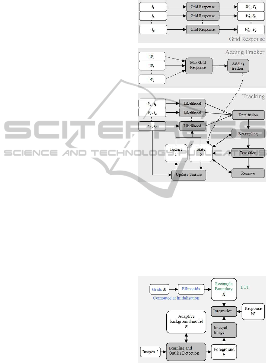
2 DETECTION AND TRACKING
Our framework includes subject detection and track-
ing in a network of cameras. Figure 1 shows a
schematic overview in which the white blocks rep-
resent data objects and the shaded blocks are func-
tions. Input colour images, I
c
, from calibrated cam-
eras, c, are synchronized and saved to host memory.
A pixel p of the image from a camera c is denoted
by I
c,p
= (I
r
, I
g
, I
b
) and p = (p
x
, p
y
) indicates pixel
position on the image plane. For detection of a new
subject, I
c
is analyzed by a grid response function to
determine W
c
= (w
1
, . . . , w
g
), where g is a grid in-
dex. This can activate and initiate an available tracker.
Once detected and a tracker activated, control then
passes to the tracking filter shown in the lower part
of Figure 1. We now explain the detection (by grid
response) and tracking functions in more detail.
2.1 Detection: The Grid Response
Function
The ’grid’ is a uniformly distributed set of 2D points
on the ground plane m
g
= (x, y), where subscript g is
grid index g = 1, 2, . . . , g
max
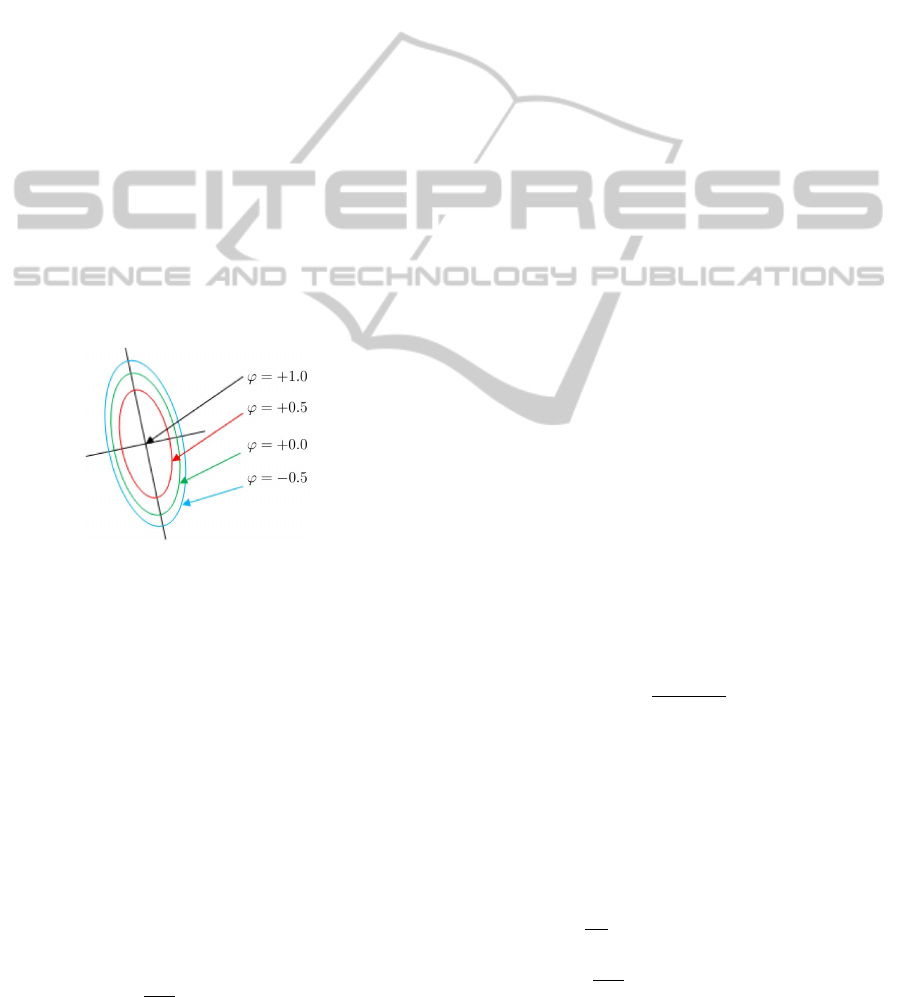
. The objective is to de-
termine the response at each grid position, as shown
Figure 1: Overall processes from top to bottom are grid re-
sponse preprocessing, adding tracker and tracking module.
in Figures 2 and 3. An ellipsoidal template of a per-
son is projected onto the image plane at each point.
From the projected ellipse in section 2.3.3, a rectangu-
lar bounding block r
g
= (p
1
, p
2
, p
3
, p
4
) is calculated.
As the cameras are fixed and pre-calibrated, the set of
grid positions, M = (m
1
, . . . , m
g
) and of rectangular
boundaries R = (r
1
, . . . , r
g
) for any camera are pre-
computed and saved in a look up table.
Figure 2: Internal structure of a grid response preprocessing
unit in Figure 1.
VISAPP 2012 - International Conference on Computer Vision Theory and Applications
226

To detect a subject, we employ a background
model, computed from I. The color distribution
of each background pixel is estimated from an ex-
tended version of an adaptiveGaussian mixture model
(Stauffer and Grimson, 1999). For a particular pixel,
this is B
p
= (µ
r
, σ
r
, µ
g
, σ
g
, µ
b
, σ
b
). The confidence in-
tervals for the background observation data are de-
fined by the chi-square test with 3 degrees of free-
dom at p-value 0.05 significance, confidence interval
Q < 7.82. Any pixel that lies out of this confidence in-
terval is classified as foreground and saved to a binary
foreground image F.
Given a rectangular boundary R in the look up ta-
ble and the foreground image F, we determine the
grid detection response w
g
as described by (Viola and
Jones, 2001; Derpanis, 2007). The integral image J
must be calculated first then the detection response
w
g
is computed from J and r
g
, where r
g
is the set of
corners {p
1
, p
2
, p
3
, p
4
} as in (Viola and Jones, 2001).
w
g
=
1
4h
x
h
y
[J(p
1
) − J(p
2
) − J(p
3
) + J(p
4
)] (1)
where J is the integral image.
J(p
x
, p
y
) =
p
y
∑
y=1
p
x
∑
x=1
F(p
x
, p
y
) (2)
The detection response w
g
of a camera c is added into
the detection response pool W
c
= (w
1
, w
2
, . . . , w
g
).
Then the global maximum response is selected and
added to the list of current subjects by the Adding
Tracker function.
Figure 3: Grids (red dots ) are projected on foreground im-
age. Detection responses are represented by green circles.
2.2 Adding a Tracker
The maximum value in the detection response pool
is selected. This maximum is verified by an empiri-
cal threshold at a fill-in ratio of 6.5 (typically between
0.6 and 0.8) as a trade off between missing a subject
and the false alarm rate. A verified maximum grid
response initiates a new tracker. A grid response in
close proximity to a current tracker is excluded to pre-
vent repeated detection.
When a new tracker is activated, a corresponding
set of states, S = {s
k,1
, s
k,2
, . . . , s
k,n
}, is initialized. A
single state, s
k,n
consists of position, velocity, height,
visibility, persistence and ID,
s
k,n
= [(Pos) (Vel) (Ht) (Vis) (Per) (ID)] (3)
where n and k are the particle and tracker indices re-
spectively. The position of all particles is set to the
grid location. The velocity is uniformly distributed in
all directions, with a uniform distribution of magni-
tude, in the absence of prior knowledge. The height of
all particles is set to an average human height of 1.7m.
The visibility and persistence are set to 1 and a unique
ID is generated. The latter variables are used in track-
ing to allow for short period disappearance due to oc-
clusion.
As stated earlier, we introduce a textured approach
based on the projection of an ellipsoid as a target sig-
nature, using a similar pixel-wise adaptive Gaussian
texture model to the background signature. At the de-
tection stage, the texture is unknown. Thus the vari-
ance of the distribution is set to a maximum and the
mean to a mid value.
2.3 Tracking using a Particle Filter
Methodology
We use a SIR (sequential importance resampling) par-
ticle filter to perform sequential Bayesian estimation.
This involves three functions: likelihood, resampling
and transition.
Let X = {x
1
, x
2
, . . .} be an observable set of data
and s
n
is a state. Note that replacing density func-
tion parameter with s
n
requires fundamental property
of particular measurement. In our case we use cam-
era model to transform s
n
to density parameters on
the image plane. The basic Bayesian equation of the
particle filter methodology is given by
P(s
n
|X) ∝ P(s
n
).P(X|s
n
). (4)
The probability P(s
n
) and collection of many states,
S = {s
n
;n = 1, 2, . . .}, form a non-parametric repre-
sentation of the prior density. A state s
n
is a coordi-
nate in a multi-dimensional state space. The coordi-
nate is a point and is called a particle. We can repre-
sent a probability density function by points and den-
sity values. This non-parametric representation re-
quires many particles to produce accurate estimation.
The particle representation is also used for expressing
another two terms, P(X|s
n
) and P(s
n
|X). The like-
lihood P(X|s
n
) is the probability of the observations
ACCELERATED PEOPLE TRACKING USING TEXTURE IN A CAMERA NETWORK
227

X being measured with given state s
n
. The product
of the prior P(s
n
) and the likelihood P(X|s
n
) forms a
posterior P(s
n
|X).
The particles are re-sampled, where the number
of offspring at the parent coordinate is proportional
to the posterior. The re-sampling makes all parti-
cles have the same weight. The offspring particles
are transformed by a stochastic transition function and
Markov model to generate the prior of the next frame.
For a comprehensive description of the operation
of the particle filter the reader is referred to the ex-
cellent text by (Ristic et al., 2004). In this paper, we
describe only the details of our own implementation,
including the contributed texture learning and track-
ing, and the accelerated implementation.
2.3.1 Transition
The transition function transforms the posterior in
the previous frame to a prior density in a succeeding
frame by an assumption of continuous motion with a
noise perturbation model. In our tracking algorithm,
we can use simple equations of motion of subjects
on the ground plane with some perturbation to model
progression from frame to frame of the video se-
quence. The stochastic equations Eq5 and Eq6 show
the propagation of a particle S
k,n
, where W is a Wiener
process, which generates standard Gaussian noise in
a stochastic model, and ∆ is the time interval between
the previous and current observation.
(Vel)
t
= (Vel)
t− 1
+ σ
vel
∆
3
2
W (5)
(Pos)
t
= (Pos)
t− 1
+ ∆(Vel)
t− 1
+ σ
pos
∆
1
2
W (6)
(Ht)
t
= (Ht)
t
+ σ
ht
∆
1
2
W (7)
Acceleration is modelled as a Wiener process,
which has a high probability to keep the previous ve-
locity. The square root of ∆ is a scaling factor of the
Wiener process. Position is the integral of velocity
over time and has some small noise due to observa-
tion. In our experiments σ
pos
is small compared to
σ
vel
. We also allow height to vary slightly over time.
Figure 4: Markov chain model of visibility state.
The visibility (Vis) is modeled as a Markov chain
as shown in the Figure 4. The visibility state has a
probability 0.25 to switch between states. In equilib-
rium, the numbers of visible and invisible particles are
equal. All invisible particles get a small constant like-
lihood. When a target is occluded, the likelihood of
a visible state is low due to lack of observation. The
invisibility state dominates and Bayesian interference
generates pressure on the probability density forcing
particles to change from visible into invisible states.
When particles are in an invisible state the persistence
level decreases.
The transition function for persistence (Per) does
not include noise, depending on the previous (Per)
and current (Vis) states. The visibility (Vis) can be
positive or negative, and its integration over time is
persistence (Per).
(Per)
t
= (Per)
t− 1
+ ∆(Vis)
t
(8)
Persistence allows the system to estimate the exis-
tence level of a target. If a target disappears, (Per)
reduces. When (Per) is below a threshold, it is rea-
sonable to assume that the target is no longer visible.
This could be due to occlusion or leaving the scene.
2.3.2 The Likelihood Function
The likelihood function, L, is the probability of occur-
rence of an observation configuration {x
1
, x
2
, . . . , x
N
}
given the prior probability density g(x, θ), where pa-
rameter θ is known a-priori. We define the observa-
tion density function f(x) from the observation set
and Eq.10 can be solved by Monte Carlo numerical
integration and log-likelihood can be written as the
integral transform in Eq.11, where log[g(x, θ)] is the
integral kernel. The kernel integral transform and log-
likelihood are analogous. Both are maximized when
f(x) and g(x, θ) are perfectly matched.
L =
∏
i
g(x
i
, θ) (9)
log[L] =
∑
i
log[g(x
i
, θ)] (10)
log[L] = N
Z
f(x). log[g(x, θ)] dx (11)
Therefore, the likelihood weight can be computed
from the kernel integral.
2.3.3 The Ellipse Kernel
Eberly (Eberly, 1999) has shown the projection of a
3D ellipsoid to a 2D ellipse function. We express this
function as a contour ϕ in Eq12, and use ϕ as an in-
tegral kernel to calculate the log-likelihood. This in-
tegrates the camera models into the projection frame-
work.
VISAPP 2012 - International Conference on Computer Vision Theory and Applications
228

ϕ = 1− A(p
x
− c
x
)
2
− B(p
x
− c
x
)(p
y
− c
y
) −C(p
y
− c
y
)
2
(12)
From camera calibration we know camera matrix K,
rotation matrix R and translation vector T. We cal-
culate eyepoint e from Eq13. The direction vector
d = (d
x
, d
y
, d
z
), which passes through e and the pixel
p = (p
x
, p
y
, 1) is computed from Eq14.
e = −R
T
T (13)
d = R
T
K
−1
p (14)
Note that Eq14 is not normalized. We insert e and
d into Eberly’s projection framework to calculate a
set of arbitrary constants (c
x
, c
y
, A, B,C) in Eq12. The
size and position of the ellipsoid are also used in con-
tour calculation. Given pixel coordinate p = (p
x
, p
y
)
we can compute contour ϕ(p) and the contour level
is used in order to determine bounding block of target
and penalty function.
To estimate and evaluate the texture of the ellip-
soid, we have to map a pixel p to a coordinate on el-
lipsoid surface q = (z, θ). The intersection between
a ray and an ellipsoid is described by (Schneider and
Eberly, 2003). The ellipsoid is scaled to a unit sphere
and the intersection point is mapped to q.
Figure 5: An ellipse contour function derived from a ellip-
soid Eq12.
Given the ray traced mapping between the image
surface and the ellipsoid surface that represents the
bounding surface of the tracked target, we now de-
scribe the formation of the likelihood function.
2.3.4 Silhouette Likelihood
Given a foreground image F and a kernel ϕ
k,n
which
is derived from state s
k,n
, we estimate the silhouette
log-likelihood λ
s
by the inner product of Eq11. As-
suming a normal distribution of foregroundpixels, the
log of the normal density is the ellipse contour func-
tion. Thus, the kernel function is constructed from ϕ
in Eq12.
λ
s
k,n
(S) =
2
πab
ϕ=1
Z
ϕ=ε
ϕ
k,n
(p)F(p) dp (15)
The log-likelihood is the summation of the prod-
uct of ϕ and F in the boundary ε < ϕ(p) < 1. The
boundary can be adjusted by setting ε as in Fig.5. Set-
ting ε=0 is insensitive to misalignment. The tracking
estimate tends to drifts away from the camera because
of perspective effect. An ellipsoid further away from
the camera generates a smaller ellipse on image plane,
which requires a smaller number of foreground pix-
els to fill it in. This means the smaller (further) el-
lipse has high probability to be completely filled than
the larger (closer) ellipse. To reduce this bias we set
larger boundary, ε = −0.5, as it creates a negative
value for any mis-aligned pixel. The silhouette likeli-
hood is very robust in the case where targets are well
separated, but is unable to handle overlaps between
targets.
2.3.5 Distraction Suppression
A major problem in multiple target tracking is dis-
traction when subjects are close on the image plane.
We use the ellipse contour function as a membership
probability, forming a penalty function to suppress
distraction.
The membership probability is defined as the as-
sociation between the observed foreground pixels and
the projected ellipse. When two or more ellipses over-
lap, any foregroundpixel possibly contributesto those
ellipses. The membership probability is a decreasing
function of the number of ellipse layers covering a
particular foreground pixel. The pixel ownership can
be calculated from the value ϕ, given the ellipse pa-
rameters and pixel location p.
Let the kernel function ϕ
k,n
(p) be a function of the
state of tracker k and pixel position p. The member-
ship probability of pixel p belonging to ellipse k of
particle n is denoted by m
k,n
(p). This depends on the
state of all active trackers i.
m
k,n
(p) =
H
k.n
(p)
∑
∀i
H
i,n
(p)
(16)
H
k,n
(p) =

1 if ϕ
k,n
(p) > ε
0 otherwise
(17)
The membership probability m suppresses distrac-
tion by penalising any pixel in the overlapping area.
The penalty factor prevents many ellipses form col-
lapsing into a single target at an early stage of inter-
action. The integral in Eq15 can be written as a sum
in Eq18, where
2
πab
is a normalizing factor.
λ
s
k,n
=
2
πab
∑
p;ε<ϕ
k,n
(p)<1
m
k,n
ϕ
k,n
F (18)
ACCELERATED PEOPLE TRACKING USING TEXTURE IN A CAMERA NETWORK
229

The likelihood of mutual overlappingsubjects is re-
duced by the penalty factor. The use of the penalty
provides distraction suppression without joint state
vectors of all subjects. The penalty prevents distrac-
tion as similar to a joint likelihood approximation
while tracker are overlapping and returns independent
likelihood in well separated targets. The approach de-
scribed here returns high accuracy with a fixed num-
ber of particles.
2.3.6 Texture Estimation and Likelihood
Our texture model is a 2D image wrapped around
the ellipsoid surface of the state vector. Each pixel
on the image contains colour distribution. Given the
camera parameters and estimated state, we can map
from pixel p on the image plane to a particular sur-
face coordinate q. The ellipsoid is scaled to a unit
sphere and a point on this sphere is expressed in coor-
dinates q = (θ, z), as this generates a uniform distribu-
tion (Weisstein, 1999), where z is the vertical axis and
θ is the azimuth. The q : (θ, z) can be mapped to an
observation image coordinate p = (p
x
, p
y
). In order
to register an observed subject to the textures surface,
we assume the facing angle is the direction of subject
movement.
Each texture pixel model, T(q), has a multivari-
ate 3D Gaussian distribution. T(q) = (µ, Σ, ω), where
µ, Σ and ω are the mean of colour vector, covari-
ance matrix and confidence, respectively. To estimate
the pixel values, each observation I(p) is used to re-
cursively update the texture model T(q). First, p is
mapped to q as described in section 2.3.3. Second,
I(p) is tested by the chi-square test given model T(q)
as the colour distribution. At p-value 0.01 the confi-
dence interval of matching between I(p) and T(q) is
Q < 11.34, where
Q = (I
p
− µ)
T
Σ
−1
(I
p
− µ), (19)
I
p
is the observation vector at p. If the observation
is in the confidence interval, the confidence ω is in-
creased, updating the texture model T(q) as Eq 20-22.
If beyond the confidence interval, ω is decreased and
T(q) is maintained. When ω drops below a threshold
the texture model is reset by setting the mean to a mid
value with large covariance.
d
q
= µ
q
− I
p
(20)
µ
q,t
= (ρ− 1)µ
q,t−1
+ ρd
q
(21)
Σ
q,t
= (ρ− 1)Σ
q,t−1
+ ρd
T
q
d
q
+ c (22)
Perspective projection means that q may be
mapped to many p. The number of observation pix-
els per texture model depends linearly on the size of
the ellipse. To avoid over fitting, the learning rate ρ
is scaled down by the size of ellipse. Hence, the new
leaning rate is ρ =
ρ
′
ab
,where ρ
′
is the original learn-
ing rate and a, b are the ellipse radii. Each tracker k
has a separate texture model T
k
.
During tracking, to compute the texture likeli-
hood, we classify an observation pixel as matched to
the texture model or not by checking the Q value,
where Q < 2.37 is a matching threshold at p-value
0.5. Any matched observation contributes to the log-
likelihood λ
t
.
λ
t
k
=
1
πab
∑
p;ϕ
k
(p)>0
D(p) (23)
D(p) =

1 if Q < 2.37
0 otherwise
(24)
The final likelihood w for a single camera c is a
function of both silhouette and texture likelihood as
in Eq25. At the early stages of tracking we have an
inadequate information of texture. The sensitivity α
t
is set to 0 to disable texture likelihood and it will be
enabled when reliable texture is obtained by checking
the covariance of the texture model is getting smaller
than a threshold.
w
c,k,n
= exp[−α
s
(λ
s
k,n
− 1)
2
+ α
t
λ
t
k,n
] (25)
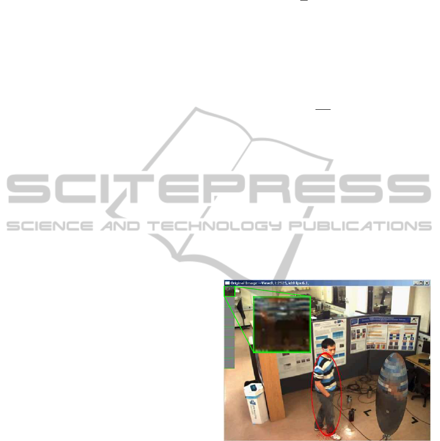
Figure 6: The posterior density of position is represented
by particles on ground plane and the red ellipse shows the
estimated result. The mean of texture obtained during track-
ing, shown in the top-left panel, is mapped to the ellipsoid
surface.
2.4 Combining Data from Multiple
Cameras
Thus far, we have described the tracking framework
form the perspective of a single camera. In our net-
work model, a subject can be seen by many cameras
so we need to combine the likelihood values from all
VISAPP 2012 - International Conference on Computer Vision Theory and Applications
230

the cameras into single global likelihood. The cam-
eras are installed at different places and their observ-
able areas may or may not overlap. A likelihood
weight w
c,k,n
from particle n of tracker k of camera
c may possibly be zero due to the target being out-
side the detectable zone or occlusion. So, validating
each camera likelihood must be done before combin-
ing these to compute a global likelihood.
Visibility on a subject can be measured form the
average weight ¯w
c,k
of all particles. The average
weight of single subject must be greater than a thresh-
old α
w
All trusted measurements are combined into
global likelihood W
k,n
.
W
k,n
=
∏
∀c
w
∗
c,k,n
(26)
where w
∗
c,k,n
is filtered weight determined from
confidence in likelihood measurement.
w
∗
c,k,n
=

w
c,k,n
if ¯w
c,k
> α
w
1 otherwise
(27)
¯w
c,k
=
1
N
∑
∀n
w
c,k,n
(28)
2.5 Removing a Tracker
A tracker may be discontinued for three reasons:
• if the persistence is zero because a target has not
reappeared in an expected time;
• if the variance of the state distribution is very
high, which happens when the tracker is distracted
by another target or there is lack of observation.
This leads to high uncertainty of estimation so we
withdraw the tracker;
• two or more trackers may be distracted and fol-
low the same target. The target which has smaller
likelihood will be terminated. Multiple trackers
following a single target can be detected by calcu-
lating the distance between the expected states.
3 IMPLEMENTATION
The particle filter approach has high complexity
which may be mitigated by using multiple processors.
Alternatives include multiple nodes on a cluster, mul-
tiple cores on a single platform or specialised hard-
ware. A very promising technology for image pro-
cessing is found in graphics processing units (GPUs)
in standard grahics cards. For example in (Boyer
et al., 2009; Zechner and Granitzer, 2009) a graphic
card provides additional speed up from 10 to 50 times.
This technology requires a developer to design an al-
gorithm in parallel to achieve full utilization.
We have implemented our system on a graphic
processing unit (GPU) GTS250 from NVIDIA using
CUDA tools for programming and optimization. The
GPU has 16 stream multiprocessors (SMs), where
each SM contains 8 stream processors. Overall, there
are 128 cores able to process concurrently and each
core has a 1.62GHz clock frequency. The cores are
controlled by the host CPU. A set of instructions is
transfered from the CPU to GPU and then all the cores
produce threds to process the same instruction with
different input data, in the SIMT (single instruction
multi thread) model. We have implemented our sys-
tem using CUDA (NVIDIA, 2010), a C like language
for graphic card programming.
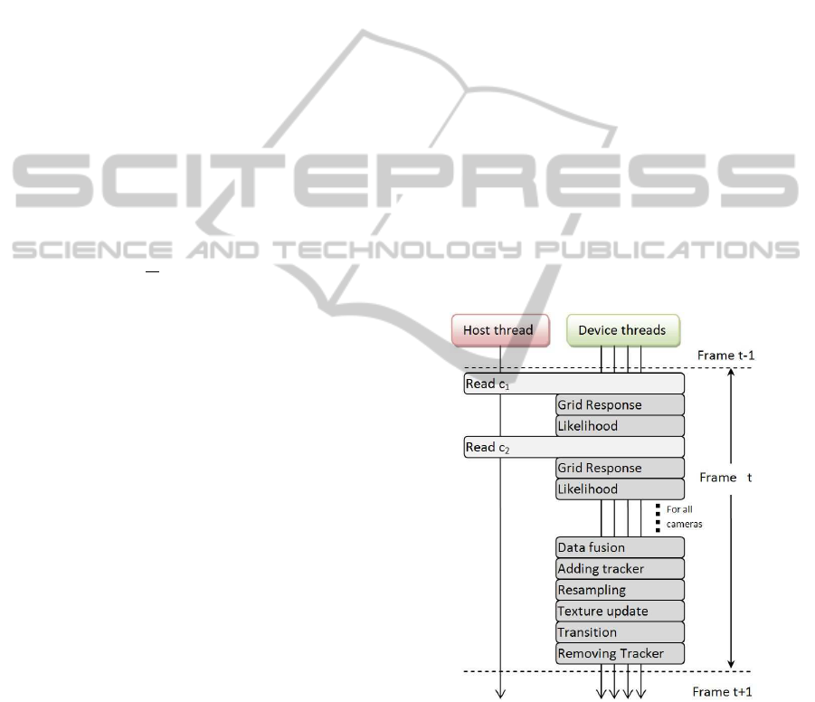
The tracking algorithm in Fig.1 can be divided
into a sequence of functions as in Fig.7. A function
is then divided into smaller pieces based on the num-
ber of output elements. Each output element is saved
to global memory on the GPU and waits for the next
execution cycle. In the implementation we also use
texture and restrict memory to accelerate data trans-
fer.
Figure 7: Main loop sequence diagram.
4 EXPERIMENT AND RESULT
We have tested the system in both off-line and in real-
time modes. In off-line mode, images were saved to
the hard-drive and loaded frame-by-frame while per-
forming tracking.
The result was evaluated by MOTA (Bernardin
ACCELERATED PEOPLE TRACKING USING TEXTURE IN A CAMERA NETWORK
231

and Stiefelhagen, 2008) (Multiple object tracking ac-
curacy), a standard metric for multi-target tracking,
MOTA = 1−
∑
t
( f
t
+ m
t
+ s
t
)
∑
t
g
t
(29)
,where f
t
, m
t
and s
t
are the number of false alarms,
miss detection and switch-id in frame t and g
t
is the
total number of targets in the scene at framet. Specifi-
cally, miss detection is when a target appears in one or
more camera views but the system fails to detect the
target. A False alarm is when a tracker is active but
there is no target associated with the tracker. Switch-
ID is an event when a target gets a new tracker ID
resulting from losing the ability to track (excluding
miss detection). Causes of Switch-ID are false-alarm,
distraction, reappearance or occlusion.
4.1 PETS09 Results
The PETS09 dataset (Ferryman and Shahrokni, 2009)
provides camera parameters and image sequences
captured from 7 different cameras. We chose the first
two views to test our algorithm. The image resolu-
tion is 768×576 pixels. To study the effect of texture
likelihood we tested the algorithm with likelihood dis-
abled and enabled. the number of particles is fixed at
512. The experiment was repeated 10 times with dif-
ferent random seed numbers. Table 1 shows that the
result of tracking without texture information has an
average MOTA of 86.5%. While using texture the av-
erage MOTA is 90.7%.
Table 3 shows time profiling on particular func-
tions. From the table we can see significant speedup
in Preprocessing, GridResponse, AddTracker and
Likelihood. In particular, the acceleration of the
Preprocess function is from 514ms to 16ms, giving
around 32 times speed up. This is because the pro-
cess can be divided into a large number of indepen-
dent pixel-wise tasks. During the Preprocess the uti-
lization of cores is restricted to 40%. Using the CUDA
Occupancy Calculator identifies a problem of lack of
local shared memory and registers. We could improve
utilization by dividing the process into further succes-
sive sub-functions.
In the Likelihood function we have 512 particles
per tracker and need about 8KB of memory. By split-
ting the computation according to the number of par-
ticles we can also reduce the computation time from
346ms to 32ms. Processor utilization is about 17%,
due to using local memory. The occupancy is fairly
small. However large numbers of cores (128 cores)
can improve the speed of the Likelihood about 10
times.
Overall, there is around 10 times speedup for the
whole process.
Table 1: Result from tracking without texture likelihood.
f(%) m(%) s(%) MOTA(%)
7.16±5.33 5.83±2.60 0.46±0.37 86.5
Table 2: Result when texture likelihood is enabled.
f(%) m(%) s(%) MOTA(%)
5.20±3.64 3.76±1.48 0.26±0.14 90.7
Table 3: Comparison of average subtotal time for single
time frame between CPU and GPU.
Function(call) CPU
time
GPU
time
Speed-
up
Util
(%)
Read(2) 36.0 40.0 0.9 -
Preprocess(2) 514.0 16.0 32.1 40
GridResponse(2) 60.0 3.6 16.7 33
Likelihood(2) 346.0 32.0 10.8 17
DataFusion(2) 4.0 1.0 4.0 4
AddTracker 45.0 2.7 16.7 33
Resample 4.0 0.5 8.0 4
TextureUpdate(2) 70.0 7.6 9.2 20
Transition 5.0 3.3 1.5 4
RemoveTracker 1.0 1.0 1.0 10
Total time (ms) 1085.0 107.7 10.1
4.2 Real-time Test Results
For on-line testing we have used 3 Point Grey Flea2
cameras connected to the computer via a 1394b hub,
which is installed on a PCI Express slot on the host
platform. This configuration can capture images from
different views in synchrony. All images pass directly
from the host to the GPU at a frame rate of 7.5 multi-
views per second. All cameras are static and well cal-
ibrated. The resulting MOTA is about 90% which is
the same as for the PETS09 data set. Some result im-
ages are shown in Fig9.
5 CONCLUSIONS AND FUTURE
WORK
Our algorithm provides a tracking accuracy MOTA of
about 90%, offering improvements on other methods
e.g. 75% in (Berclaz et al., 2009) and 80% in (Bre-
itenstein et al., 2010). From our results, augmenting
the image with texture information reduces the error
rate from 13.5% to 9.3%.
The penalty function makes a hybrid estimation
using independent and joint posterior densities. The
estimation suppresses mutual distraction resulting in
VISAPP 2012 - International Conference on Computer Vision Theory and Applications
232

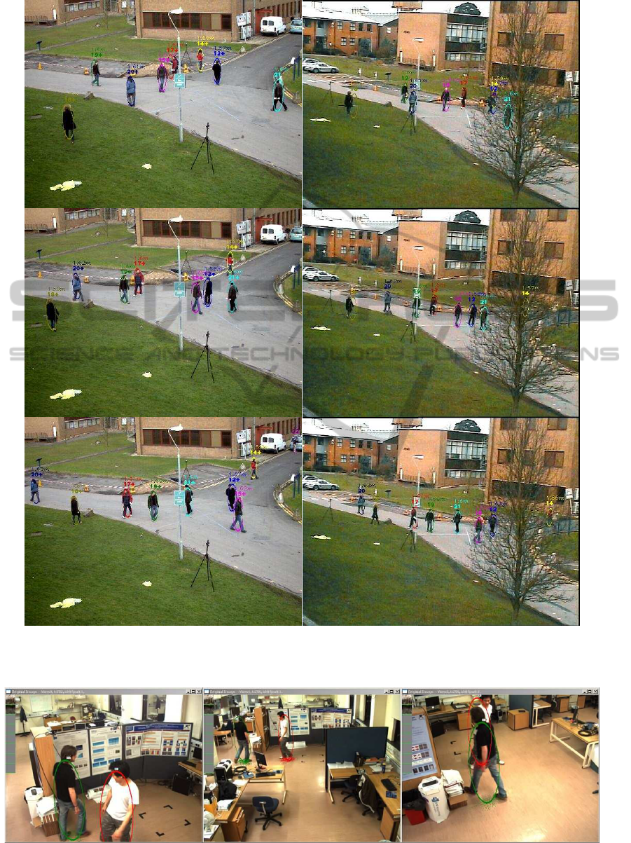
Figure 8: Evaluating with PET09 dataset. First and second columns are result sequences from camera1 and camera3, from
top to bottom are frame 700, 720 and 740, respectively. The numbers over ellipse show ID and height in unit meter.
Figure 9: The ellipses show estimated positions projected on each view and panel on top-left are texture images of the subjects.
ACCELERATED PEOPLE TRACKING USING TEXTURE IN A CAMERA NETWORK
233

improved accuracy in the early tracking stage.
We have gained significant speedup by deploying
parallel processing on the GPU, from 1 frame per sec-
ond to 10 frames per second which is broadly com-
parable to current standard CCTV installations. This
allows near-real-time tracking of large numbers of ob-
jects.
We will next investigate further improvements to
our implementation to optimise thread occupancy on
the GPU. In the longer term we will explore real
time object tracking between non-overlapping cam-
eras where we think our texture approach will im-
prove object handover.
REFERENCES
An, K. H. and Chung, M. J. (2008). 3d head tracking and
pose-robust 2d texture map-based face recognition us-
ing a simple ellipsoid model. In Proc. IEEE/RSJ
Int. Conf. Intelligent Robots and Systems IROS 2008,
pages 307–312.
Bardet, F. and Chateau, T. (2008). Mcmc particle filter for
real-time visual tracking of vehicles. In Proc. 11th
International IEEE Conference on Intelligent Trans-
portation Systems ITSC 2008, pages 539–544.
Berclaz, J., Fleuret, F., and Fua, P. (2009). Multiple ob-
ject tracking using flow linear programming. In Proc.
Twelfth IEEE Int Performance Evaluation of Tracking
and Surveillance (PETS-Winter) Workshop, pages 1–
8.
Bernardin, K. and Stiefelhagen, R. (2008). Evaluating mul-
tiple object tracking performance: the clear mot met-
rics. J. Image Video Process., 2008:1–10.
Boyer, M., Tarjan, D., Acton, S. T., and Skadron, K. (2009).
Accelerating leukocyte tracking using cuda: A case
study in leveraging manycore coprocessors. In Proc.
IEEE International Symposium on Parallel & Dis-
tributed Processing IPDPS 2009, pages 1–12.
Breitenstein, M., Reichlin, F., Leibe, B., Koller-Meier,
E., and Van Gool, L. (2010). Online multi-
person tracking-by-detection from a single, uncali-
brated camera. PAMI. Early Access.
del Blanco, C. R., Mohedano, R., Garcia, N., Salgado,
L., and Jaureguizar, F. (2008). Color-based 3d par-
ticle filtering for robust tracking in heterogeneous en-
vironments. In Proc. Second ACM/IEEE International
Conference on Distributed Smart Cameras ICDSC
2008, pages 1–10.
Derpanis, K. G. (2007). Integral image-based representa-
tions. Department of Computer Science and Engineer-
ing York University Paper.
Deutscher, J., Blake, A., and Reid, I. (2000). Articulated
body motion capture by annealed particle filtering.
In Proc. IEEE Conf. Computer Vision and Pattern
Recognition, volume 2, pages 126–133.
Eberly, D. (1999). Perspective projection of an ellipse.
www.geometrictools.com.
Ferryman, J. and Shahrokni, A. (2009). Pets2009: Dataset
and challenge. In Proc. Twelfth IEEE Int Per-
formance Evaluation of Tracking and Surveillance
(PETS-Winter) Workshop, pages 1–6.
Husz, Z. L., Wallace, A. M., and Green, P. R. (2011). Track-
ing with a hierarchical partitioned particle filter and
movement modelling. SMCB, pages 1–14. Early Ac-
cess.
Isard, M. and Blake, A. (1996). Contour tracking by
stochastic propagation of conditional density. In
ECCV ’96: Proceedings of the 4th European Confer-
ence on Computer Vision-Volume I, pages 343–356,
London, UK. Springer-Verlag.
Jaward, M., Mihaylova, L., Canagarajah, N., and Bull, D.
(2006). Multiple object tracking using particle filters.
In Aerospace Conference, 2006 IEEE, page 8 pp.
Kreucher, C., Kastella, K., and Hero, A. O. (2005). Mul-
titarget tracking using the joint multitarget probability
density. AES, 41(4):1396–1414.
NVIDIA (2010). Nvidia cuda c best practice guide.
Peursum, P., Venkatesh, S., and West, G. (2007). Tracking-
as-recognition for articulated full-body human motion
analysis. In Proc. IEEE Conference on Computer Vi-
sion and Pattern Recognition CVPR ’07, pages 1–8.
Ristic, B., Arulampalam, S., and Gordon, N. (2004). Be-
yound the Kalman Filter Particle Filter for Tracking
Application. DSTO.
Schneider, P. J. and Eberly, D. H. (2003). Geometric Tools
for Computer Graphics. Elsevier.
Sidenbladh, H., De la Torre, F., and Black, M. J. (2000).
A framework for modeling the appearance of 3d ar-
ticulated figures. In Proc. Fourth IEEE International
Conference on Automatic Face and Gesture Recogni-
tion, pages 368–375.
Stauffer, C. and Grimson, W. E. L. (1999). Adaptive back-
ground mixture models for real time tracking. In Proc.
IEEE Computer Society Conference on. Computer Vi-
sion and Pattern Recognition, volume 2, page 252 Vol.
2.
Vezzani, R., Grana, C., and Cucchiara, R. (2011). Prob-
abilistic people tracking with appearance models and
occlusion classification: The AD-HOC system. Pat-
tern Recognition Letters, 32(6):867–877.
Viola, P. and Jones, M. (2001). Rapid object detection using
a boosted cascade of simple features. In Proc. IEEE
Computer Society Conf. Computer Vision and Pattern
Recognition CVPR 2001, volume 1.
Weisstein, E. (1999). Sphere point picking. From
MathWorld–A Wolfram Web Resource.
Zechner, M. and Granitzer, M. (2009). Accelerating k-
means on the graphics processor via cuda. In Proc.
First International Conference on Intensive Applica-
tions and Services INTENSIVE ’09, pages 7–15.
VISAPP 2012 - International Conference on Computer Vision Theory and Applications
234