A FORMAL METHOD FOR SCHEDULING ANALYSIS

OF A PARTITIONED MULTIPROCESSOR SYSTEM

Dynamic Priority Time Petri Nets

Walid Karamti, Adel Mahfoudhi, Yessine Hadj Kacem and Mohamed Abid

CES Laboratory, ENIS Soukra km 3,5, University of Sfax, B.P.:w 1173-3000 Sfax, Tunisia

Keywords:

Real-time System, Petri Nets, dPTPN, Scheduling Analysis, Least Laxity First.

Abstract:

In order to examine whether the timing constraints of a Real-Time application are met, we propose an ex-

tension of Time Petri Nets model that takes into account the scheduling of a set of tasks distributed over a

multiprocessor architecture. This paper is concerned with dynamic Priority-driven scheduling, whose policy

is known to be supported by a new formalism called dynamic Priority Time Petri Nets (dPTPN). Its ultimate

objective is to show how to deal with the Least Laxity First Scheduling policy with a set of periodic inde-

pendent tasks. Besides, the use of dynamic priorities gives a determinism aspect to the model in which a

crossing of concurrent transitions exists. Therefore, the execution of the model is accelerated and the number

of accessible states is decreased.

1 INTRODUCTION

Real-time systems (RTS) are characterized by com-

plex applications that require powerful architectures

to satisfy them. The trend is to use multiprocessor

architectures, among which we can distinguish the

presence of two families of multiprocessor schedul-

ing. The ﬁrst is the family of global scheduling in

which each task of application can migrate among the

processor resources to be executed. The major draw-

back of the global family is the absence of an optimal

scheduling algorithm (Kwang and Leung, 1988). The

second family is the partitioned scheduling, in which

one task of the application can be executed on a sin-

gle processor resource. It is to bring the multipro-

cessor scheduling problem in uniprocessor schedul-

ing problems in which there exist optimal scheduling

algorithms (Liu and Layland, 1973). The family of

partitioned scheduling involves two steps; a step of

assigning tasks to processors, and another for analyz-

ing the scheduling of each partition (Sha et al., 2004).

It is important to detect errors of scheduling as early

as possible in order to minimize the costs for its cor-

rection. The analytical techniques used are based on

the analytical work of Liu and Layland (Liu and Lay-

land, 1973).

The speciﬁcation with formal methods could be

able to reduce the problem impact. In fact, it repre-

sents a recent research area in order to develop a con-

sistent approach. Starting from an abstract modeling

that takes into account a set of constraints, the main

objective of this technique is to determine and check

the system properties.

Many varieties of formal methods exist and the

choice of the appropriate one depends on the char-

acteristics of the system and the properties to be

checked. Deductive reasoning and model checking

are two major categories of proving methods. Using

the deductivemethod, a speciﬁcation gives an abstract

description of the signiﬁcant behavior of the required

system. This behavior is checked for the deﬁned im-

plementation through the proving of theorems which

constitute the rules of reﬁnement. The major limita-

tion of this category is that the user interacting with

the prover must be able to guide him.

1.1 Related Work

The technique of model checking is of an irrefutable

advantage, allowing early and economical detection

of errors at an early stage of the design process. This

explains the growing popularity it enjoys in the indus-

trial world.

Aiming at developing a system model, designers

must ensure a sufﬁcient accuracy to preserve all the

properties for check and a level of abstraction ap-

propriate not to penalize the analysis phase. There

are many formalisms proposed for modeling real-time

317

Karamti W., Mahfoudhi A., Hadj Kacem Y. and Abid M..

A FORMAL METHOD FOR SCHEDULING ANALYSIS OF A PARTITIONED MULTIPROCESSOR SYSTEM - Dynamic Priority Time Petri Nets.

DOI: 10.5220/0003809103170326

In Proceedings of the 2nd International Conference on Pervasive Embedded Computing and Communication Systems (PECCS-2012), pages 317-326

ISBN: 978-989-8565-00-6

 2012 SCITEPRESS (Science and Technology Publications, Lda.)

systems. Each one has its speciﬁc characteristics,

more or less relevant in a speciﬁc design and accord-

ing to the type of analysis considered.

Time, parallel processing and synchronization

are primordial characteristics for scheduling analy-

sis. Compared with other formalisms, the Time

Petri Nets (TPNs) (Merlin, 1974) can easily support

these features without leading to combinatorial ex-

plosion. Therefore, TPNs face problems when mod-

eling a scheduling policy. Indeed, TPNs is a non-

deterministic formalism because when two or more

transitions are enabled it is not speciﬁed which one

has to ﬁre. In reverse, the scheduling algorithm al-

ways chooses an event from the available ones ac-

cording to a deﬁned policy. Several extensions have

been created to support scheduling policy by adding

priorities to transitions.

It should be born in mind that the absence of a

TPNs extension supports dynamic priorities. That is

why we detail the extensions with static priority used

for scheduling analysis.

Roux (Roux and D´eplanche, 2002) presented an

STPN (Scheduling Timed Petri Nets) to analyze peri-

odic tasks on a multiprocessor architecture. The pri-

orities were introduced by the inhibitor arcs to sup-

port a ﬁxed priority driven scheduling policy such

as RM (Rate Monotonic) (Liu and Layland, 1973).

The contribution of his proposal lies in the calcula-

tion of a reduced state space compared to that evoked

by (Berthomieu and Diaz, 1991). Such proposal was

improved by (Lime and Roux, 2004) and (Lime and

Roux, 2009) to support the tasks with variable time

execution.

The STPN (Roux and D´eplanche, 2002) adds con-

straints on the crossing of the transitions to check the

respect for the ﬁring interval. Therefore, the check

of these constraints is a new dimension added to the

problem of scheduling analysis.

Berthomieu (Berthomieu et al., 2006)in his turn

utilized the inhibitor arcs to introduce the notion of

priorities within the Petri nets through the extension

of PrTPNs (Priority Time Petri Nets). His proposal

was based on a method of temporal analysis of the

network. Indeed, from a sequence of non-temporal

transitions, his method was to recover the possible du-

rations between the ﬁring of transitions in order. The

durations are the solutions of a linear programming

problem.

Both of PrTPN and STPN are TPNs extensions, so

they retain these properties, i.e., the indeterminacy of

the date of crossing of an event. However the model-

ing of a scheduling policy of a hard real-time system

requires that all dates used are determined. The pri-

ority is modeled through the inhibitors arcs added as

new components to those of PNs. The RTS modeling

with Petri nets gives rise to the models that are often

complex. Moreover, the addition of an inhibitor arc

makes the model more complex and therefore the ex-

traction of properties becomes more difﬁcult.

A new extension PTPN (Priority Time Petri Nets) was

proposed in (Kacem et al., 2010), in which a crossing

date is associated with each temporal event. In fact,

a transition is valid when the clock shows the date

of ﬁring. In addition, PTPN uses a new method of

priorities integration to address the problem of tran-

sitions conﬂict. In this method, a priority is inserted

on the input arcs of the dependent transitions (Kacem

et al., 2010).Moreover, this method allows to mas-

ter the complexity of the PTPN model by eliminat-

ing the use of another component, such as inhibitor

arcs, to specify priorities. To control the size of the

PTPN model, a hierarchical modeling was proposed

in (Mahfoudhi et al., 2011).

1.2 Contribution and Outline of the

Paper

Most of the Time Petri Nets extensions dedicated for

scheduling analysis such as PrTPN (Berthomieu et al.,

2006), STPN (Roux and D´eplanche, 2002) and PTPN

(Kacem et al., 2010) use a ﬁxed priority. However,

the use of a ﬁxed priority allows the covering of a re-

duced space of RTS such as periodic tasks and ﬁxed

Priority-driven scheduling strategies.

On a single processor platform, the LLF (Least

Laxity First) scheduling policy, a dynamic Priority-

driven scheduling, is known as the most general algo-

rithm on RTS. It is proven as an optimal preemptive

scheduling algorithm (Goossens et al., 2004). How-

ever, its features upon multiprocessor platforms have

been little studied so far.

In this paper, we account for the scheduling anal-

ysis of multiprocessor system via a new extension of

Time Petri Nets. The major advantageof the proposed

extension is that it gives a solution to the modeling

and analysis of a dynamic priority-driven scheduling

policy (LLF) taking into account periodic indepen-

dent system tasks partitioned over a multiprocessor

platforms.

The present paper is organized as follows. Firstly,

the deﬁnitions and execution semantics of the pro-

posed dynamic Priority Petri Nets (dPTPN) are

overviewed in section 2. Next, section 3 shows how

our extended formalism is used for specifying the

scheduling analysis problem through experiments. Fi-

nally, the proposed approach is brieﬂy outlined and

future perspectives are given.

PECCS 2012 - International Conference on Pervasive and Embedded Computing and Communication Systems

318

2 DYNAMIC PRIORITY TIME

PETRI NETS: dPTPN

Our challenge is the integration of a dynamic-Priority

driven scheduling policy in Petri Nets. This strategy

is based on the dynamic calculation of priorities. In-

deed, the value of a priority changes at runtime.

In the standard PN, the events (transitions) had the

same grade of emergency. Thus when transitions con-

ﬂict, there are no favorable transition to cross before

the others. Accordingly, the semantics of the standard

PN does not support a scheduling policy.

A real-time scheduling policy is characterized by

a sequence of timed events and no events conﬂict. To

reach our goal, we will integrate these two features in

PN. To do so, we distinguish between temporal events

and concurrent events that are sources of conﬂict. We

propose a new extension of PN with two types of tran-

sitions T (temporal transitions) and T

(compound

transition Fig. 1).

Figure 1: T

compound.

The latter is all about a transition with a prepro-

cessing that precedes the crossing to calculate its pri-

ority. Indeed, if two Tcp transitions are enabled and

share at least a place in entry then the preprocessing is

made to determine the transition which will be ﬁred,

with a priority changing according to the state of the

network described by the marking M. By analogy in

real-time scheduling with dynamic priorities such as

LLF, the priority changes according to laxity.

In this section, we present the syntax of the

new Petri Net extension (dynamic priority Petri Nets

dPTPN) as well as its ﬁring semantics. The simula-

tion of the sequences of ﬁring is then explained.

2.1 Syntax

A Petri Nets (Petri, 1962) can be deﬁned as 4-uplet :

PN = hP, T, B, Fi (1)

, where:

(1) P = {p

, p

, ..., p

} is a ﬁnite set of places n > 0;

(2) T = {t

, t

, ..., t

} is a ﬁnite set of transition m > 0

(3) B : (P× T) 7→ N is the backward incidence func-

tion;

(4) F : (P × T) 7→ N is the forward incidence func-

tion;

Each system state is represented by a marking M of

the net and deﬁned by : M : P 7→ N.

The dPTPN is deﬁned by the 7-uplet :

dPTPN =



PN,T

,coef, M



(2)

(1) PN: is a Petri Net;

(2) T



,··· ,T



: is a ﬁnite set of com-

pound transition k > 0;

(3) T

: T 7→ Q

is the ﬁring time of a transition.

∀t ∈ T, t is a temporal transition ⇐⇒ T

(t) 6= 0.If

(t) = 0 then t is an immediate transition. Each

temporal transition t is coupled with a local clock

(Hl(t)),with Hl : T −→ Q

(4) B

: (P × T

) 7→ N is the backward incidence

function associated with compound transition;

(5) F

: (P × T

) 7→ N is the forward incidence

function associated with compound transition;

(6) coe f : (P× T

) 7→ Z is the coefﬁcient function

associated with compound transition;

(7) M

: is the initial marking;

2.2 Semantics

To deal with the problem of the state space explo-

sion, it is worthwhile to mention the contribution of

the methods considered as partial order (Antti, 1989)

(Kimmo, 1994) (Buy and Sloan, 1994) building on a

relation of equivalence between various sequences of

possible ﬁrings, starting from the same state. In fact,

when two sequences are found to be equivalent, then

only one of them is selected. This relation of equiva-

lence is based on the notion of independence of tran-

sitions. Two transitions are independent if they are

not in the same neighborhood (see eq. 9).

Based on the approach of partial order and the T

compound, dPTPN relies on a well-deﬁned strategy

for the ﬁring during a conﬂict of transitions. The strat-

egy builds on the construction of a sequence of the

highest priority and valid transitions dFT

. For the ﬁr-

ing of a marking M, dPTPN offersa machine of ﬁring

called dPTPN Firing Machine dPFM, whose mecha-

nism is described in Fig. 2. The entry of the machine

dPFM is a marking M of the dPTPN network. For

each entry, the machine builds the dFT

set, which

consists of two sub-sets FT

and FT

, which in turn

present the ﬁring transitions of T and those of T

, re-

spectively. When it is about a marking dead-end, the

dFT

set is empty (FT

is empty and FT

is empty)

and the dPFM machine stops.

The modeling of an RTS with dPTPN distin-

guishes between the temporal and immediate events.

To do so, the machine dPFM supplies a chain of pro-

cessing. Indeed, the machine, ﬁrstly, determines the

valid temporal transitions set VT

from the FT

set,

A FORMAL METHOD FOR SCHEDULING ANALYSIS OF A PARTITIONED MULTIPROCESSOR SYSTEM -

Dynamic Priority Time Petri Nets

319

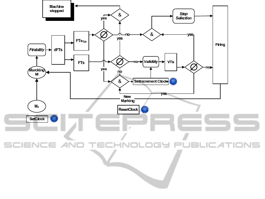
Figure 2: dPTPN ﬁring machine.

and secondly, the VT

is analyzed. The machine ﬁres

any valid transition before passing to the following

stage and for each ﬁring the dFT

is reconstructed

(FT

and FT

, respectively). The last stage con-

sists in solving the problem of conﬂict by choosing

among the compound transitions with the highest pri-

ority that will be ﬁred.

All immediate transitions must be crossed before

the analysis of FT

. In fact, the immediate transi-

tions are more urgent and their ﬁring can give birth to

a marking that presents a new conﬂict of transitions.

2.2.1 Firability

dFT

presents the enabled transitions set. In fact,

dFT

is the union of the enabled temporal transi-

tions set FT

and the enabled compound transitions

set FT

dFT

= FT

∪ FT

. (3)

let t ∈ T,t ∈ dFT

⇔ t ∈ FT

∨t ∈ FT

(4)

with



= {t ∈ T/B( . ,t) ≤ M}



t ∈ T/B

( . ,t) ≤ M



For each subset FT

and FT

is associated with a

function indicator χ

and χ

: T −→ {0,1} (5)

x 7−→



1 if x ∈ FT

0 otherwise

: T −→ {0,1} (6)

x 7−→



1 if x ∈ FT

0 otherwise

2.2.2 Validity

A transition is valid if it is enabled and respects its

ﬁring date. We should bear in mind that T

is an

immediate transition. Therefore, we deﬁne the Valid

Transition Set (VT

) as a subset of FT

(VT

⊆ FT



t ∈ FT

/Hl(t) = T

(t)



(7)

is the function indicator of VT

with:

: FT

−→ {0,1} (8)

The main advantage of utilization of the T

compo-

nent is to solve the problem of transition conﬂict. The

best way is to select the T

transition having the high-

est priority.

2.2.3 Step Selection

∀T

∈ T

, T

is selected if and only if it is enabled

and has the highest priority compared with its neigh-

borhood. First of all we present the neighborhood of

transition T

∀T

∈ T

is a neighbor o f T

⇔ ∃p ∈ P such that B



p,T



6= 0∧ B



p,T



6= 0

(9)

We consider a matrix N

to indicate the neighborhood

of all transitions T

compared to each place P:

: T

× P −→ {0,1} (10)

, p) 7−→



1 if B

(p,t

) > 0

0 otherwise

PECCS 2012 - International Conference on Pervasive and Embedded Computing and Communication Systems

320

Three steps are applied to select the transition that

has the highest priority. The ﬁrst step is the calcula-

tion of the priority for each enabled transition T

. In

fact, the priority depends on the state of the dPTPN

model and the matrix coef. Each T

calculate its pri-

ority using the scalar product of coef matrix with the

marking vector M.

Prio : FT

−→ Z (11)

7−→ hcoef (.,t

)| Mi

In the second step, we mark the corresponding pri-

orities to each T

neighborhood. More precisely we

deﬁne the following function:

Prod : FT

× P 7→ Z (12)

, p) 7−→ Prio(t

, p)

the third step, the transition having the highest priority

per palce is selected from the vector Prod(., p

Min : P −→ FT

(13)

p 7−→ t

with {∀t

6= t

, Prod (t

, p) < Prod(t

, p)}

Finally, the FT

must be updated to present only the

selected transitions: ∀t

∈ T

,∀p ∈ P,

Prod(t

, p) 6= 0∧ t

6= Min(p) =⇒ χ

) = 0

(14)

2.2.4 Firing

We deﬁne the ﬁring of a given FT vector. In dPTPN,

FT can be an VT

vector or an FT

vector:

∀FT ∈

,FT

,Firing(FT) =⇒











FT = VT

⇔ M

′

= M +

∑

t∈FT

(F (.,t) − B(.,t))

FT = FT

⇔ M

′

= M +

∑

t∈FT



(.,t) − B

(.,t)



(15)

2.2.5 Clocks Management

According to dPTPN, the clocks management abides

some rules, which are:

Rule1 (Set): When a transition is enabled, for its ﬁrst

time, then its matching clock is activated and initial-

ized with zero.

Rule2 (Reset): After ﬁring VT

, the clocks of valid

transitions will reset.

Rule3 (Increment Clock): The clock of a transition

is incrementing if the transition is enabled, no valid

transition exists and the FT

is empty.

SetIncremetClock() is activated ⇐⇒

6= ⊘ ∧ FT

= ⊘ ∧VT

= ⊘ (16)

2.2.6 dPTPN State Graph

In dPTPN, a state is a node composed of (M,tmp),

where M is a marking andtmp is the time for its ﬁring.

The state graph SG is deﬁned by: SG = hS, Ai with:

• S: is a set of state;

• A : S × S −→ dFT

: presents the arcs connecting

the reachable states. The connection arcs will be

established only when two markings of two states

are reachable via dFT

vector.

The process of construction of the states graph cor-

responds to the execution of the Algorithm 1. In-

deed, it deals with a repetitive execution of the dPFM

machine and for every iteration a new state is con-

structed.

During the ﬁrst tic of the clock associated with

Algorithm 1: State graph construction.

1: M: Marking

2: dFT

: enabled transitions set

3: FT

: enabled temporal transitions set

4: VT

: valid temporal transitions set

5: Hl: clocks set

6: FT

: enabled compound transitions set

7: initializeMarking(M)

8: SetClock(Hl)

9: StateConstruction(M)

10: while M ≺ B and M ≺ B

11: Firability(dFT

)

12: FT

← temporalTransition(dFT

)

13: FT

← CompoundTransition(dFT

)

14: if FT

6= ⊘ then

15: VT

← Validity(FT

)

16: if VT

6= ⊘ then

17: Firing(VT

)

18: StateConstruction(M)

19: ResetClock(Hl(VT

))

20: else if FT

= ⊘ then

21: SetIncrementClock(Hl(FT

))

22: end if

23: else if FT

6= ⊘ then

24: StepSelection(FT

)

25: Firing(dFT

)

26: StateConstruction(M)

27: end if

28: end while

dPTPN, the marking M is initialized by the initialize-

Marking(M) function and the ﬁrst state is built by the

function

StateConstruction(M)

. The process of con-

struction starts with applying an iterative work. For

each iteration, the machine dPFM begins with the de-

termination of the ﬁred transitions in the vector dFT

by applying the function Firability(dFT

). Vectors

and FT

are initialized from dFT

to distin-

guish between the temporal transitions and the T

A FORMAL METHOD FOR SCHEDULING ANALYSIS OF A PARTITIONED MULTIPROCESSOR SYSTEM -

Dynamic Priority Time Petri Nets

321

transitions.

The validation of the temporal transitions is an-

alyzed via the function Validity(FT

). To check the

existence of the valid transitions, a conditional struc-

ture appears to ﬁre them at once. However, the ab-

sence of the valid transitions allows us to check the

existence of the compound transitions. The presence

of the transitions in FT

requires a selection of the

highest priority to ﬁre it. Any ﬁring leads to an update

of the marking M and a construction of a new state to

connect it with the precedent one through a weight arc

dFT

The absence of the valid transitions and the com-

pound transitions leads to an incrementation of the

global clock of the dPTPN by calling the function

SetIncrementClock(). This process is repeated as long

as the marking M satisﬁes at least a transition. The

Process ends as soon as it is in a marking dead-end or

during a reset of the marking.

3 MODEL CONSTRUCTION

The RTS Ω is deﬁned by the 3-uplet:

Ω = hTask, Proc, Alloci (17)

with:

(1) Task : is a ﬁnite set of real-time tasks with each

Task

∈ Task determined by

Task

= hR

, P

, D

, C

i (18)

• R

: the date of the ﬁrst activation.

• P

: the period associated with the task.

• D

: the deadline associated with the task, we con-

sider an RTS with P

= D

• C

: the execution period of the task for the P

pe-

riod.

(2) Proc : a ﬁnite set of processors.

(3) Alloc : Task 7→ Proc, a function which allocates a

task to a processor. Alloc is a surjective function. In

fact a processor is allocated to at least one task. But a

task must be assigned to only one processor.

∀t

∈ Task, ∀P

∈ Proc,

Alloc(t

) = P

∧ Alloc(t

) = P

⇒ P

= P

(19)

To model the system Ω with the new dPTPN exten-

sion, we specify each component of Ω. The model of

scheduling analysis is described through the commu-

nication between the various Task and Proc compo-

nents. Each processor is modelled by a simple place,

whose marking describes the state of the resource.

The presence of a mark indicates that the resource is

free and ready to execute a task. The absence of the

mark indicates that the resource is occupied by a sys-

tem task Ω.

3.1 Task Model

The modeling can be divided into two major patterns.

The ﬁrst one pertains to the notion of creation, activa-

tion and deadline, as for the second, it describes the

concept of execution task.

3.1.1 Creation, Activation and Deadline

At ﬁrst, a task Task

∈ Task is created. For a date

”Ri”, the creation is made, leading to the passage of

the task towards the created state. So, the period ”Pi”

starts. As shown in Fig. 3, each state is modelled by

a place and every event by a transition. When it is

about an event accompanied with a date of progress,

the transition will take a date of ﬁring similar to that

of the event. When it is about a non-created state, it is

presented by a marked place (UnCreated). The cre-

ation is modelled by a temporal transition Creation

which takes a date of ”Ri” ﬁring.

When the local clock of Hl(Creation) indicates

the date of ﬁring R

, the transition is then valid

and the ﬁring allows to register a mark in the place

Created and P

tokens in RemainingPeriod. Indeed,

the marking of the place Created shows that the

task is created and P

marks present the remaining

duration before the deadline. For each tic of the

global clock of the dPTPN, the transition IncPeriod

is validated. Besides, its ﬁring leads to a decre-

mentation of the remaining duration before the dead-

line and an incrementation of the exhausted time of

the period. When Pi tokens are moved towards the

place ElapsedPeriod, the period is exhausted and a

new period must be activated. The event of activa-

tion is modelled by a transition Restart, whose ﬁr-

ing activates a new period by depositing P

marks

in RemainingPeriod and the creation of a new in-

stance of the task by putting down a token in the place

Created.

Figure 3: Creation, activation and deadline.

We present a ﬁrst scenario in which the ﬁrst acti-

vation of the task Task

exists. We will then introduce

PECCS 2012 - International Conference on Pervasive and Embedded Computing and Communication Systems

322

a scenario of deadline event provided with the mech-

anism of its detection by the model dPTPN.

The place Created indicates the presence of a

mark. To model the activation of the ﬁrst instance

of the task, we use a mutual exclusion described by

two places Disabled and Activated. According to

the initial scenario, the ﬁrst instance of the task is

deactivated, where from the presence of a token in

Disabled. The current marking allows the ﬁring of

the transition Activation and the ﬁring allows the sup-

ply of a mark in places Ready and Activated. The cur-

rent state proves that the current instance of the task

is activated and lends itself to be run on the processor

resource.

With regard to the second scenario, it describes

the activation of a new period while the old instance

of the task has not ﬁnished its execution yet. The

model presents a mark in the place Created and an-

other in the place Activated. This marking allows the

ﬁring of the transition Activation for the activation of

the new instance and the transition Tdeadline to in-

dicate that the task overtook its deadline. The ﬁring

of Tdeadline allows the registration of a mark in the

place Deadline and the blocking of the entire model

dPTPN of the task.

3.1.2 Execution

The execution of a task is described by two main

events, the ﬁrst of which pertains to the allocation of

the resource processor and the second represents the

execution of the task on the processor.

The resource processor is a resource shared be-

tween the various tasks of the same partition, and for

a given moment, a single task occupies it. The alloca-

tion of the processor depends on the used scheduling

strategy. In our study we are interested in the strategy

based on LLF.

With dPTPN, each task calls for the resource pro-

cessor if and only if it presents a mark in the place

Ready. So, the event of allocation is modeled by

a transition allocation of the type T

. The proces-

sor will be attributed to the task having the transition

allocation with the highest priority (having the least

laxity). Indeed, the allocation is modeled by a regis-

tration of a mark in the place getProc. Fig. 4 illus-

trates two requests of allocation of the processor P1

by two tasks (Alloc(Task1)=Alloc(Task2)=P1).

Fig. 4 shows that for each task, there are 4 places

and a T

transition type as well as a place for model-

ing the processor. Both transitions T1allocation and

T2allocation that are ﬁred by the current marking are

in conﬂict because of the shared place P1. The prior-

ities of the transitions will be calculated according to

the LLF policy. In fact, the LLF makes its schedul-

Figure 4: Allocation processor.

ing decisions based on the maximum time span that a

request can tolerate before being picked up for execu-

tion.

The laxity of a request at any given moment is the

time span that it can tolerate before the time it has

to be picked up for execution; otherwise its deadline

will deﬁnitely be missed. As a request is being exe-

cuted, its laxity does not change. However, the laxity

of a task decreases as the request waits (either in the

ready-to-run queue or elsewhere).Its chances of being

overrun increase. When the laxity of a task becomes

zero, it can no longer tolerate waiting.

The laxity of a task is a dynamic value that

changes as the circumstances change. Four values af-

fect its computation:(1) the absolute time of the mo-

ment when we want to compute the laxity of the task,

t,(2) the absolute value of the deadline of this request,

,(3) the execution time of this request, C

, and (4)

the execution time that has been spent on this request

since it was generated, e

. The following is the simple

formula for computing the laxity of a request with the

aforementioned values.

L = (D

− t) − (C

− e

) (20)

In Fig. 5, the (D

−t) value is presented with the mark-

ing of the place ”RemainingPeriod” and the (C

− e

)

is presented with the marking of the place ”C

”.

The main interest of ”coef” matrix is to provide

a solution for presenting the arithmetic operators. In-

deed, to model the equation L with dPTPN, we in-

tercalate the coefﬁcient ”1” on the arc connecting the

place ”RemainingPeriod” and the T

and ”2” on the

arc between the place ”C

” and ”T

”.

The marking of the model Fig. 4 presents

4 marks in T

RemainingPeriod and 2 marks in

RemainingPeriod. The T

allocation transition is

the most priority because it has the least laxity (L=2-

1=1). The ﬁring of T2alloctaion involves the extrac-

tion of two marks of P1 and T

Ready and a registra-

tion of a mark in T

getProc to indicate that the pro-

cessor P1 is attributed to task

. The place T

Ready

always remains marked because task

is always pend-

A FORMAL METHOD FOR SCHEDULING ANALYSIS OF A PARTITIONED MULTIPROCESSOR SYSTEM -

Dynamic Priority Time Petri Nets

323

Figure 5: Execution.

ing to the processor P1.

As soon as the marking of the model indicates the

presence of a mark in the place getProc (Fig.5), the

task begins the execution by ﬁring the immediate tran-

sition execution.

It is worthwhile to mention that the interest of the

present paper is the preemptive systems. Indeed, to

manage the modeling of this type of problem, we pro-

pose that each task occupies the processor during only

one unit of time then releases it. The corresponding

dPTPN model is described by a temporal transition

incrementing with a date of ﬁring equal to 1. The ﬁr-

ing of this event allows not only the removal of a mark

from the place Ci and one from the place InExec but

also the registration of a mark in the place maker as

well as the incrementation of the tokens of ei by an-

other mark. Such incrementation indicates that the

task ended a unit of execution during the period Pi.

It should be noted that there is an emergence of

three events endCi, endDeadline and RelaxProc. We

consider the scenario when the three events are en-

abled.

The place maker is a shared place between those

events. So they are modeled with T

transitions and

are in the same neighborhood. We must specify the

priority of each transition for solving the conﬂict. The

current scenario shows that the task has completed its

Ci units and the deadline is triggered. In the schedul-

ing analysis, this scenario is not considered as non-

schedulable task. Thus, the priority of the endCi tran-

sition is higher than endDeadline. To do so, we at-

tribute the coefﬁcients ”3” to the input arc of endCi

and ”2” to the input arc of ”endDeadline”.

The non-schedulablesystem is described when the

endDeadline and RelaxProc are enabled. It means

that a new period is triggered when the last period is

still activated. Since, the endDeadline must be ﬁred

immediately, we must attribute the higher priority to

it and a smaller priority to RelaxProc (coef=1).

3.2 Case Study

In the present section, we introduce the technique of

how dPTPN solve the scheduling analysis problems

of the real-time systems. It is through a case study

that our dPTPN extension is brought to the light.

In fact, we present a generic experiment which

consists of a non-schedulable system. In the latter, we

establish how the way how the evolution of dPTPN

model supplies a description of the temporal fault to

help the designers in reﬁning the partitioning space

Sw/Hw. It should be born in mind that due to space

limitation, we present a pedagogical experiment.

The case study deals with three tasks running

on two processors. Using deﬁnition 17, the spec-

iﬁcations of the task characteristics as well as the

allocation of the processors by the tasks are described

as follows.

Task = {T1(0, 16,16,4), T2(0,8, 8,2), T3(0,4,4, 2),

T4(0,6, 6,4), T5(0,7,7, 4)};

Proc = {P1, P2};

Alloc(T1) = P1 Alloc(T4) = P2

Alloc(T2) = P1 Alloc(T5) = P2

Alloc(T3) = P1

The ﬁrst stage consists in modeling of Ω with the

dPTPN. As for the second step, it consists in placing

the marks on dPTPN constituents: a mark in each

constituent ”Processor: P1, P2”. A mark in the places

”Uncreated” and ”Disabled” of ”Task : T1, T2, T3,

T4, T5”. We also place 4, 2, 2, 4 and 4 marks on the

places ”Ci” of tasks T1, T2, T3, T4 and T5 respec-

tively.

At this level, let us recall that the strength of our

dPTPN extension is its capacity to determine step by

step the valid scheduling sequence. In fact, the exe-

cution of the model based on dPFM allows the con-

struction of the valid sequence. If the construction is

well established, then the system is well scheduled,

otherwise when the sequence encounters a marking,

then the system is considered as non-schedulable.

Moreover, the supplied scheduling sequence is opti-

mal because dPTPN supports the optimal dynamic

priority LLF strategy.

For a better presentation, we have detailed the ex-

ecution of the model in Table 1. Three columns are

represented; the ﬁrst ”step” is the number of the steps

in the scheduling, which corresponds to a state in the

states graph explained previously. The ﬁrst step starts

with ”step=0”. The second column is ”time”; it is the

PECCS 2012 - International Conference on Pervasive and Embedded Computing and Communication Systems

324

Table 1: Model execution related to the case study.

Step Time

dFT

Step Time

dFT

0 0 Creating(T1,T2,T3,T4,T5) −− 20 4 Restart(T3) −−

1 0 Activation(T1,T2,T3,T4,T5) −− 21 4 Activation(T3) −−

2 0 ⊘ Allocation(T1,T2,T3,T4,T5) 22 4 ⊘ RelaxProc(T2,T5)

EndCi(T2)

3 1 Execution(T3,T4) −− 23 4 Releasing(T2,T5) −−

4 1 Incrementing(T3,T4) −− 24 4 ⊘ Allocation(T1,T3,T4)

IncPeriod(T1,T2,T3,T4,T5)

5 1 ⊘ RelaxProc(T3,T4) 25 4 Execution(T3,T4) −−

6 1 Releasing(T3,T4) −− 26 5 Incrementing(T3,T4) −−

IncPeriod(T1,T2,T3,T4,T5)

7 1 ⊘ Allocation(T1,T2,T3,T4,T5) 27 5 ⊘ RelaxProc(T3,T4)

8 1 Execution(T3,T5) −− 28 5 Releasing(T3,T5) −−

9 2 Incrementing(T3,T5) −− 29 5 ⊘ Allocation(T1,T3,T4)

IncPeriod(T1,T2,T3,T4,T5)

10 2 ⊘ RelaxProc(T3,T5) 30 5 Execution(T3,T4) −−

EndCi(T3)

11 2 Releasing(T3,T5) −− 31 6 Incrementing(T3,T4) −−

IncPeriod(T1,T2,T3,T4,T5)

12 2 ⊘ Allocation(T1,T2,T4,T5) 32 6 Restart(T4) −−

RelaxProc(T3,T4)

13 2 Execution(T2,T4) −− 33 6 ⊘ EndDealine(T4)

EndCi(T3,T4)

14 3 Incrementing(T2,T4) −− 34 6 Releasing(T3,T4) −−

IncPeriod(T1,T2,T3,T4,T5)

15 3 ⊘ RelaxProc(T2,T4) 35 6 ⊘ Allocation(T1,T4,T5)

16 3 Releasing(T2,T4) −− 36 6 Execution(T1,T5) −−

17 3 ⊘ Allocation(T1,T2,T4,T5) 37 7 Incrementing(T3,T5) −−

IncPeriod(T1,T2,T3,T4,T5)

18 3 Execution(T2,T5) −− 38 7 Restart(T5) −−

19 4 Incrementing(T2,T5) −− 39 7 ⊘ RelaxProc(T1,T4)

IncPeriod(T1,T2,T3,T4,T5) EndDealine(T5)

number of tics of the global clock of the PTPN model.

The last column ”Ft

” represents the high-priority and

valid transitions in each step of scheduling.

The execution process of the model starts at time

0 with the initial marking M

. These two parame-

ters present the necessary entries to launch the dPFM

machine. Such machine determines the high-priority

and valid transitions t in the columns FT

and

: Transition-name (Task-name). It is the case

of ”step0”, in which the column FT

presents ”Cre-

ation(T1, T2,T3)” and no enabled t

exists. The si-

multaneous ﬁring of this set of events gives birth to a

new marking and a new step ”step1”.

As for ”step2”, it presents no valid temporal event

exist and the event ”Allocation(T1,T2,T3,T4,T5)” in

the column FT

. This indicates that ﬁve tasks

are ready to allocate the processors ”P1” and ”P2”.

”Allocation(T1)” and ”Allocation(T2)” and ”Alloca-

tion(T3)” belong to the same neighborhood. How-

ever, ”Allocation(T3)” has the lowest laxity (highest

priority according LLF) (l=2) . Therefore, it will be

ﬁred before ”Allocation(T1)” and ”Allocation(T2)”.

The transitions with the highest priority are presented

with the red color for each FT

What is worthy to note is that step ”step38”

presents the ”Restart(T5)” event. This indicates that

the period T5 is provoked and a new T5 instance

is created while the work of the last instance is not

achieved. The ﬁring and the passage to the step

”step39” brings about a new marking which replies

to the event ”EndDeadline(T5)”. The ﬁring of this

event implies the blocking of the execution, signaling

a temporal fault (deadline). The current marking de-

scribes the combination of tasks that causes this fault.

It will be a useful feedback to the designer to change

the allocation Task/Processor.

4 CONCLUSIONS

In this paper, we have presented a new method for

scheduling analysis of periodic tasks running on mul-

tiprocessor architecture. The analysis technique is ba-

A FORMAL METHOD FOR SCHEDULING ANALYSIS OF A PARTITIONED MULTIPROCESSOR SYSTEM -

Dynamic Priority Time Petri Nets

325

sed on proposed dynamic Priority Time Petri Nets

dPTPN. Compared to the existing research work, the

salient characteristic of novelty in dPTPN consists

in the attribution of a dynamic priority via a com-

pound transition. Therefore dPTPN supports a dy-

namic Priority-driven policy (LLF) and its seman-

tics isolate the conﬂict of enabled transitions. Rather

than presenting a solution for the problems of confu-

sion, dPTPN Firing Machine accelerates the dPTPN

evolution by applying temporal ﬁltering for temporal

transitions and priority ﬁltering for T

transitions. In

regular PN, the ﬁring of a transition requires the iden-

tiﬁcation of the new set of enabled transitions. How-

ever, with dPFM, this set is established only after the

ﬁring of the old one. It is also guided by dynamic pri-

orities. Consequently,starting from a marking M

, the

dPFM ﬁres simultaneously valid temporal transitions

and the T

having the highest priority then returns the

new marking M.

In the current paper, we deal with a partitioning

strategy of multiprocessors scheduling. This tech-

nique is concerned as a static scheduling method.

The distribution of tasks on processors is often done

through a tool based on heuristics. When the schedul-

ing analysis technique, i.e. dPTPN, detects a non-

schedulable system, then the tool generates a new so-

lution. This process causes a waste of time gener-

ating problems during implementing of the schedul-

ing strategy. However, dPTPN indicates the exact

description of the non-schedulable sequence and just

changed this sequence to obtain a valid scheduling.

This presents our challenge in future research work.

We are also interested in including performance anal-

ysis in the veriﬁcation of RTS and planning to inte-

grate dPTPN design patterns ranging building blocks

for an easy model construction and interpretation.

REFERENCES

Antti, V. (1989). Stubborn sets for reduced state space gen-

eration. In Applications and Theory of Petri Nets,

pages 491–515.

Berthomieu, B. and Diaz, M. (1991). Modeling and ver-

iﬁcation of time dependent systems using time petri

nets. IEEE Trans. Softw. Eng., 17(3):259–273.

Berthomieu, B., Peres, F., and Vernadat, F. (2006). Bridg-

ing the gap between timed automata and bounded time

petri nets. In FORMATS, pages 82–97.

Buy, U. and Sloan, R. (1994). Analysis of real-time pro-

grams with simple time petri nets. In ISSTA ’94:

Proceedings of the 1994 ACM SIGSOFT international

symposium on Software testing and analysis, pages

228–239, New York, NY, USA. ACM.

Goossens, J., Richard, P., Richard, P., and Bruxelles, U.

L. D. (2004). Overview of real-time scheduling prob-

lems. In Euro Workshop on Project Management and

Scheduling.

Kacem, Y. H., Karamti, W., Mahfoudhi, A., and Abid, M.

(2010). A petri net extension for schedulability analy-

sis of real time embedded systems. In PDPTA, pages

304–314.

Kimmo, V. (1994). On combining the stubborn set method

with the sleep set method. In Valette, R., editor, Ap-

plication and Theory of Petri Nets 1994: 15th Inter-

national Conference, Zaragoza, Spain, June 20–24,

1994, Proceedings, volume 815 of Lecture Notes in

Computer Science, pages 548–567. Springer-Verlag,

Berlin, Germany. Springer-Verlag Berlin Heidelberg

1994.

Kwang, S. H. and Leung, J.-T. (1988). On-line scheduling

of real-time tasks. In IEEE Real-Time Systems Sym-

posium, pages 244–250.

Lime, D. and Roux, O. (2004). A translation based method

for the timed analysis of scheduling extended time

petri nets. In RTSS ’04: Proceedings of the 25th IEEE

International Real-Time Systems Symposium, pages

187–196, Washington, DC, USA. IEEE Computer So-

ciety.

Lime, D. and Roux, O. H. (2009). Formal veriﬁcation of

real-time systems with preemptive scheduling. Real-

Time Syst., 41(2):118–151.

Liu, C. L. and Layland, J. W. (1973). Scheduling algo-

rithms for multiprogramming in a hard-real-time en-

vironment. J. ACM, 20:46–61.

Mahfoudhi, A., Hadj Kacem, Y., Karamti, W., and Abid,

M. (2011). Compositional speciﬁcation of real

time embedded systems by priority time petri nets.

The Journal of Supercomputing, pages 1–26. doi

10.1007/s11227-011-0557-9.

Merlin, P. M. (1974). A Study of the Recoverability of Com-

puting Systems. Irvine: Univ. California, PhD Thesis.

available from Ann Arbor: Univ Microﬁlms, No. 75–

11026.

Petri, C. A. (1962). Fundamentals of a theory of asyn-

chronous information ﬂow. In IFIP Congress, pages

386–390.

Roux, O. H. and D´eplanche, A. M. (2002). A t-time Petri

net extension for real time-task scheduling modeling.

European Journal of Automation (JESA), 36(7):973–

987.

Sha, L., Abdelzaher, T., Arz´en, K. E., Cervin, A., Baker, T.,

Burns, A., Buttazzo, G., Caccamo, M., Lehoczky, J.,

and Mok, K. A. (2004). Real time scheduling theory:

A historical perspective. Real-Time Systems, 28:101–

155. 10.1023/B:TIME.0000045315.61234.1e.

PECCS 2012 - International Conference on Pervasive and Embedded Computing and Communication Systems

326