REGULARIZED RECONSTRUCTION OF ULTRASONIC
IMAGING AND THE REGULARIZATION PARAMETER
CHOICE
Leonardo G. S. Zanin, Fábio K. Schneider and Marcelo V. W. Zibetti
Graduate School of Electrical Engineering and Computer Science, Federal University of Technology, Paraná, Brazil
Keywords: Ultrasound imaging, Inverse problems, Image reconstruction, Singular value decomposition.
Abstract: Ultrasound image reconstruction based on inverse problems has attracted attention to the ultrasonic imaging
research community recently. Different from standard beamforming-based methods techniques, this new
imaging method tries to solve a linear system g=Hf as a form of reconstructing the ultrasound image. In
order to understand the behaviour of this imaging system, it is important to analyse the forward problem. In
this paper, we analyse the effect of the noise in acquisition matrix using singular value decomposition. Also,
the effect of regularization parameter in dealing with the noise is investigated in regularized. This analysis
provides some interesting insights in the understanding of how the inverse reconstruction can be improve
some aspects higher than beamforming.
1 INTRODUCTION
Beamforming-based methods are traditionally used
to ultrasound imaging, which relies on Delay-And-
Sum (DAS) approach (Stergiopoulos, 2000). The
DAS approach provides some positive benefits such
as real-time imaging. Even though Beamforming
(BF) has had some important improvements, such as
adaptive BF (Synnevåg et al., 2007) it still has
limitations on its achieved resolution. Going further
may require new reconstruction approaches.
Some recent research such (Lavarello et al.,
2006); (Lingvall and Olofsson, 2007); (Viola et al.,
2008), proposed an ultrasonic image reconstruction
methods based on inverse problems (Barrett and
Myers, 2004). In this methodology the data
acquisition process, know as forward system, is
utilized to relate the image of a region of interest
(ROI) with the captured data-signal. The
reconstructed image is obtained by solving this
system, what is known as the inverse solution
(Barrett and Myers, 2004).
Inverse approaches can significantly reduce the
point spreading, providing a sharper image with
increased quality and resolution (Lavarello et al.,
2006); (Lingvall and Olofsson, 2007); (Viola et al.,
2008). The noise, however, may limit the potential
of the inverse reconstruction, so a proper balance
must be applied. The regularized reconstructions
(RR) treat this problem by choosing an adequate
regularization parameter (Hansen, 1998); (Vogel,
2002).
Several methods for optimal automatic
determination of this parameter exist, such as GCV
(Golub and Von Matt, 1997), L-curve and others
(Hansen, 1998). However, automatic determination
of the parameter highly increases the computational
cost of the reconstruction. Other alternatives are
prior determination of the regularization, instead of
automatic, such as the statistical methods (Bovik,
2000).
This paper proposes a combination of RR and
prior choice of the regularization parameter to
ultrasonic imaging systems. The paper is organized
as following: in Section 2, the forward system is
explained, in Section 3, the RR is presented, together
with the choice of the regularization parameter. In
Section 4, a small brief of the Singular Value
Decomposition (SVD), and the spectrums of the
image and noise are presented. The analysis of the
system for the prior choice of the regularization
parameter is presented in Section 5, together with
some samples of reconstructed images. Finely, in
Section 6, a discussion of the results and the
conclusions are drawn.
438
G. S. Zanin L., K. Schneider F. and V. W. Zibetti M..
REGULARIZED RECONSTRUCTION OF ULTRASONIC IMAGING AND THE REGULARIZATION PARAMETER CHOICE.
DOI: 10.5220/0003794904380442
In Proceedings of the International Conference on Bio-inspired Systems and Signal Processing (BIOSIGNALS-2012), pages 438-442
ISBN: 978-989-8425-89-8
Copyright
c
 2012 SCITEPRESS (Science and Technology Publications, Lda.)

2 FORWARD SYSTEM FOR
ULTRASOUND IMAGING
The investigation acoustic pulse in the spatial
position r, during a time t, is models as (Lingvall
and Olofsson, 2007):
)()(),(),(
1
tuththtp
k
ef
k
K
k
sf
k
∗∗=
∑
=
rr
(1)
In (1), its considered K elements in the ultrasound
array. The u
k
(t) is the electric signal applied to the k
th
array element, h
k
ef
(t) is the forward electro-acoustic
impulse response of the element, while the acoustic
spatial impulse response is denoted as h
k
sf
(r,t). The
pressure p(r,t) reaching a position r react according
to the reflectivity function f(r), which is the
information to be imaged. This echo signal formed
by this interaction at the position r, reaching the n
th
array element is:
)(),()(),(),( rrrr ftpththtg
eb
n
sb
nn
∗∗=
(2)
We consider that N
e
elements in the array are used
for echo recording. This returning echo is spread by
the backward spatial impulse response h
n
sb
(r,t),
reaching the sensor where it is convolved with the
backward electro-acoustic impulse response h
n
eb
(t).
Joining (1) and (2) we can express the echo from a
particular position as:
)(),(),( rrr fthtg
nn
=
(3)
where
),()(),(),( tpththth
eb
n
sb
nn
rrr ∗∗=
(4)
Considering that the data-signal g
n
(r,t) from (3) is
provided by echoes from all r positions belonging to
the Cartesian coordinates in the 2D image grid. In
this paper we assume that the discrete signal can be
represented as:
∑
∈
=
grid
inin
fthtg
r
rrr ][],[],[
(5)
The image size is M
1
×M
2
, being M=M
1
·M
2
number
of pixels. Also, t
i
is a discrete time sample being S
the total time samples from an element. Putting the
equation (5) in a matrix-vector format leads to g
n
=
H
n
f, where g
n
=[g
n
(t
1
), …, g
n
(t
S
)]
T
is a vector with all
the captured samples from the n
th
element, while
f=[f(1,1), …, f (M
1
,1), f (1,2), …, f (M
1
M
2
)]
T
is a
vector with the image pixels re-ordered.
We can join the time samples from all elements
in the form:
ηf
H
H
g
g
ηHfg +
⎥
⎥
⎥
⎦
⎤
⎢
⎢
⎢
⎣
⎡
=
⎥
⎥
⎥
⎦
⎤
⎢
⎢
⎢
⎣
⎡
=+=
NN
##
11
(6)
In (6), we have the full system. The H matrix has
size of N×M, being N=N
e
·S. The sensor response,
pulses and signal spreading are all involved to form
the matrix, so it contains the system behavior. The
noise is represented by η.
3 REGULARIZED
RECONSTRUCTION
The RR used in this paper is based on the Tikhonov
regularization for least squares (Hansen, 1998),
described as:
[
]
2
2
2
2
2
minarg)(
ˆ
fHfgf
f
αα +−=
Tik
(7)
In (7), the parameter α, known as the regularization
parameter, is real and positive (Bovik, 2000). When
α→0, the reconstructed image is usually sharp, but
noise is amplified due to the ill-conditioning of H.
Increasing the regularization parameter reduces
noise amplification, stabilizing the image. However,
it also reduces the sharpness of the solution.
The minimum of (7) is achieved when the
gradient is zero, or equivalently when:
gHfIHH
T
Tik
T
=+
ˆ
)(
2
α
(8)
This gives the following solution:
gHIHHf
TT
Tik
12
)(
ˆ
−
+= α
(9)
The reconstruction in (9) requires the inversion of
the matrix; however, this computation can be done
off-line and then stored in the ultrasound equipment
to reconstruction process. On the other hand, prior
choices of α must be defined previously to the
inverse computation.
3.1 Choice of the Regularization
Parameter
Automatic parameter selection methods, such as the
GCV (Golub and Von Matt, 1997) and the L-curve
(Hansen, 1998), are alternatives to the balance
between noise and image sharpness, but they cannot
determine the parameter a priori.
Our alternative for prior α determination requires
previous knowledge of the noise levels. Several
methods based on the knowledge of the noise and
REGULARIZED RECONSTRUCTION OF ULTRASONIC IMAGING AND THE REGULARIZATION PARAMETER
CHOICE
439

image variances exist, such as the statistical
Maximum a Posterior (MAP) estimation
(Mohammad-Djafari, 1995); (Therrien, 1992). MAP
estimation leads to a reconstruction algorithm
similar to (7), where α= δ
η
/δ
f
, being δ
η
and δ
f
the
noise and the image standard deviation respectively.
In (Hansen, 1998) it is mentioned that the
regularization is needed if the discrete Picard
condition is not achieved. In order to clearly state
the discrete Picard condition, we briefly mention the
SVD and define the spectrums of the image and
noise.
4 THE SINGULAR VALUE
ANALISIS
4.1 Singular Value Decomposition
The SVD (Barrett and Myers, 2004) is able to
reveals the spectrum of a matrix by diagonalizing it.
The spectrum shows the filtering effect of the
acquisition system. This information is similar to the
frequency response of shift invariant systems.
Utilizing the SVD, the matrix H can be
represented as:
∑
=
==
p
k
T
kkk
T
1
vuUSVH σ
(10)
Where U is a N×N matrix, V is a M×M matrix, and
S is an N×M diagonal matrix with the elements
σ
1
,
σ
2
, … , σ
p
, where p=min(N,M) in its diagonal. The
orthonormal columns v
k
represent the right singular
vectors. The orthonormal matrix V
T
transforms the
image vector f to new space where the singular
values weight this transformed image. The result is
transformed to another space by the U matrix,
constructed with orthonormal column vectors u
k
,
which
are the left singular vectors. The set { σ
k
, u
k
,
v
k
}, 1 ≤ k ≤ p, are the singular system of H.
4.2 Definition of the Spectrums of the
Image and the Noise
Using the SVD one can observe that the operation
Hf first transforms the image to the spectral space,
through V
T
f, forming the coefficients {v
k
T
f}, 1 ≤ k ≤
p, which is the unfiltered spectrum of image. In the
spectrum, the image is filtered through SV
T
f
generating the noiseless data spectrum (filtered
spectrum) defined by {σ
k
(v
k
T
f)},1 ≤ k ≤ p. The same
filtered spectrum can be obtained by U
T
Hf,
generating {u
k
T
Hf}, 1 ≤ k ≤ p, which is the same as
{σ
k
(v
k
T
f)}. Also, we can observe the filtered
spectrum with noise, resulted from g=Hf+η, by
doing U
T
g=U
T
Hf+U
T
η which is a composition of
filtered image spectrum, or U
T
Hf, and the noise
spectrum, or U
T
η, also defined as {u
k
T
η}, 1 ≤ k ≤ p.
In general, the image spectrum is relatively
arbitrary. However the filtered spectrum is more
predictable. According to the discrete Pickard
condition (Hansen, 1998), the absolute value of the
filtered image spectrum, or σ
k
|v
k
T
f|, must decay, on
average, at the same rate (or more) than the rate of
decaying of the s.v. (Hansen, 1998); (Vogel, 2002).
This behavior, which is stated for general systems, is
also observed for ultrasonic systems.
4.3 Prior Determination of the
Regularization Parameter
The regularization is needed because the inverse will
strongly amplify the components related to small
singular values. One can say those spectrum
components on elevated k positions may has more
noise than signal, while the lower k positions may
has more signal the noise.
The regularized reconstruction, expressed with
the SVD is:
∑
=
−
+
=+=
p
k
k
k
T
kk
TT
Tik
1
22
12
)(
)(
ˆ
v
gu
gHIHHf
ασ
σ
α
(11)
One can note that the RR, instead of inverting the
s.v. directly, invert the regularized s.v., or
sqrt(σ
k
2
+α
2
). This stabilizes the inverse solution,
avoiding excessive noise amplification, and corrects
the filtered signal when the signal is stronger than
noise.
Our main contribution in this paper is the
observation that the regularized s.v. must follow de
average decaying of data spectrum. The data
spectrum (noise plus filtered spectrum) follows, on
average, the regularized s.v. line, or:
22
ασ +≈
k
T
k
ogu
(12)
Considering the weighting by a constant o, the α is
δ
η
/o, which is very consistent with MAP, where the
constant o is chosen as δ
f
. So, in order to find a
reasonably regularization parameter a priori, one
may use data captured from several different study
objects, i.e. phantoms. This data can be transformed
to the spectrum, using the SVD, and an appropriate
scaling constant o can be found. One may simply
adjust the curve manually so the constant o may
provide the overlap between singular values and data
BIOSIGNALS 2012 - International Conference on Bio-inspired Systems and Signal Processing
440

spectrum, especially in the lower k components.
5 SIMULATION RESULTS
In this section, the reconstructed images with
regularized inversion using different parameters are
shown. For these experiments we used signals
generated using Field II toolbox (Jensen, 1996). For
all experiments an ultrasonic pulse of 5 MHz, with
80% of the bandwidth, sampled at 100MHz and
sound speed of c=1540 m/s were considered. The
ROI is an area of 10×10mm in which the sensor
array is 25mm from the center of the ROI in the
longitudinal dimension, and centered in the lateral
dimension. The 64 elements of the sensor are spaced
by λ=c/f. We do not use focused pulses, neither any
non-uniform apodization. The resolution grid is
60×60 pixels. Some sample figures are reconstructed
with BF and RR from (9). Also, we add a white
Gaussian noise to the signal with standard deviation
to achieve a SNR of 10dB and 20dB.
The Figure 1 has the results of the determination
of the ideal α for this system. Note that average
noise lines for both SNR of 10dB and 20dB, cross
the singular values line. This means we need to
regularize the system to avoid excessive noise
amplification. The standard deviation for the noise
and acquisition with SNR of 10 and 20dB are shown
in Table 1. By adjusting the curves the estimated
constant o is nearly to 3·10
-2
, which is close to the α
parameter suggested by MAP estimation. The
regularized curves are plotted in the Figure 1.
Table 1: Standard deviation and regularization parameter.
SNR δ
η
·(10
-11
) α·(10
-9
)
10dB 6.5652 2.1884
20dB 2.0786 0.6928
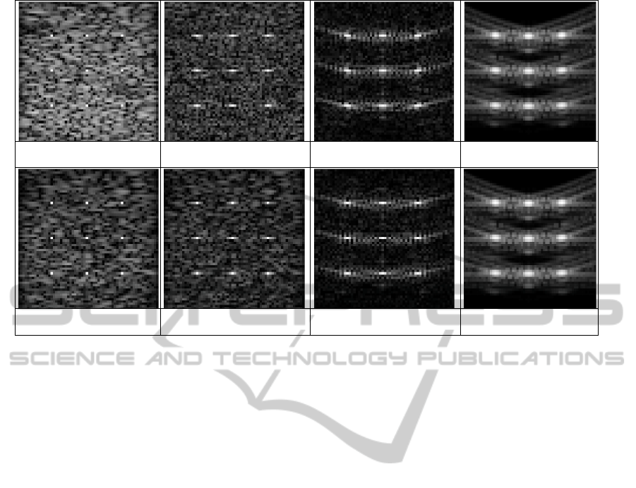
In order to compare the RR with different
parameters for both SNR's, we utilized three α
spanned by one order of magnitude above an one
order of magnitude below, i.e., α
bellow
=0.1×α, α, and
α
above
=10×α. The results are shown in Figure 2,
comparing with the BF reconstruction.
Analyzing the results, it is possible to observe in
the images reconstructed with α
bellow
, in figures 2(a)
and (e), that the noise were over amplified. With the
ideal α, the inverse results have a noise level
between the underregularized and BF. The noise was
not too much amplified and the spots are more
compact, which corresponds to an improvement in
resolution. Figures 2(c) and (g) show reconstructed
images obtained by α
above
, wich is an overregularized
inverse approach. This result is more similar to BF,
but it is possible to note that the spots are not so
spread as BF. Comparing these inverse
reconstructions with the BF, is possible to note that
the noise was amplified, but the spreading was
significantly reduced.
Figure 1: The singular values σ
k
, the average noise level
δ
η
/o, and the regularized singular values sqrt(σ
k
2
+α
2
)
adjusted for SNR of 10dB and 20dB.
6 DISCUSSIONS AND
CONCLUSIONS
This analysis evidenced the importance of choice of
regularization parameter. The higher the α, smaller
the noise and smaller the reduction of spreading; the
smaller the α, higher the correction of the spreading
under the cost of increased noise amplification. With
RR, an improvement in image resolution was
obtained when compared with DAS BF.
In this paper we also investigate how the noise
affects the ultrasound forward system through de
SVD analysis. Mainly, we use this analysis to obtain
a better regularization parameter to regularized
inverse approach. We observed some of advantage
that inverse reconstruction provides when applied to
ultrasound imaging systems. This new method, also
investigated in recent works (Lavarello et al., 2006);
(Lingvall and Olofsson, 2007); (Viola et al., 2008)
has been proven its effectiveness and is able to be
used in modern ultrasound systems.
Some of limitations existent in BF, such as the
lateral spreading of the spots are improved with this
new method. The great limitation of RR is the
computational cost and memory requirements,
which makes it, by now, impossible to be applied for
real-time imaging as BF. However their ability of
improve the ultrasound image resolution makes it
REGULARIZED RECONSTRUCTION OF ULTRASONIC IMAGING AND THE REGULARIZATION PARAMETER
CHOICE
441

(a) Underregularized with
α
b
ellow
(
10dB
)
.
(b) Regularized with α
(10dB)
. (c) Overregularized with
α
above
(
10dB
)
.
(d) DAS Beamforming.
(e) Underregularized with
α
b
ellow
(
20dB
)
.
(f) Regularized with α
(20dB)
. (g) Overregularized with
α
above
(
20dB
)
.
(h) DAS Beamforming.
Figure 2: Images obtained for reconstructions of the data with SNR of 10 (a-d) and 20dB (e-h), through the regularized
inverse, obtained from different α and DAS Beamforming.
very attractive and researches in this area must be
encouraged.
ACKNOWLEDGEMENTS
Authors thanks the Brazilian Federal Agency for
Post-Graduate Education (CAPES) for financial
support.
REFERENCES
Barrett, H. H., & Myers, K. J. M. (2004). Foundations of
Image Science. John Willey & Sons.
Bovik, A. C. (2000). Handbook of image and video
processing. Academic Press.
Golub, G. H., & Von Matt, U. (1997). Generalized cross-
validation for large-scale problems. Journal of
Computational and Graphical Statistics, 1–34.
JSTOR.
Hansen, P. C. (1998). Rank-deficient and discrete ill-
posed problems. SIAM.
Jensen, J. A. (1996). Field: A Program for Simulating
Ultrasound Systems Field: A Program for Simulating
Ultrasound Systems. Medical & Biological
Engineering & Computing (Vol. 34, pp. 351- 353).
Lavarello, R. J., Kamalabadi, F., & O’Brien, W. D.
(2006). A Regularized Inverse Approach to Ultrasonic
Pulse-Echo Imaging. IEEE Transactions on Medical
Imaging, 25(6), 712-22.
Lingvall, F., & Olofsson, T. (2007). On time-domain
model-based ultrasonic array imaging. IEEE
Transactions on Ultrasonics, Ferroelectrics and
Frequency Control, 54(8), 1623-33.
Mohammad-Djafari, A. (1995). A full Bayesian approach
for inverse problems. International Workshop on
Maximum Entropy and Bayesian Methods, 135-144.
Stergiopoulos, S. (2000). Advanced Signal Processing
Handbook: Theory and Implementation for Radar,
Sonar, and Medical Imaging Real Time Systems.
Abingdon: CRC Press.
Synnevåg, J.-F., Austeng, A., & Holm, S. (2007).
Adaptive Beamforming Applied to Medical
Ultrasound Imaging. IEEE Transactions on
Ultrasonics, Ferroelectrics and Frequency Control,
54(8), 1606-13.
Therrien, C. W. (1992). Discrete Random Signals and
Statistical Signal Processing. Prentice Hall.
Viola, F., Ellis, M., & Walker, W. F. (2008). Time-domain
optimized near-field estimator for ultrasound imaging:
initial development and results. IEEE Transactions on
Medical Imaging, 27(1), 99-110.
doi:10.1109/TMI.2007.903579
Vogel, C. R. (2002). Computational Methods for Inverse
Problems. SIAM.
BIOSIGNALS 2012 - International Conference on Bio-inspired Systems and Signal Processing
442