DIVISIVE MONOTHETIC CLUSTERING

FOR INTERVAL AND HISTOGRAM-VALUED DATA

Paula Brito

and Marie Chavent

Faculdade de Economia & LIAAD-INESC Porto LA, Universidade do Porto, Porto, Portugal

UFR Sciences et Mod

elisation, IMB et INRIA CQFD, Universit

e de Bordeaux 2, Bordeaux, France

Keywords:

Divisive clustering, Histogram data, Interval data, Monothetic clustering.

Abstract:

In this paper we propose a divisive top-down clustering method designed for interval and histogram-valued

data. The method provides a hierarchy on a set of objects together with a monothetic characterization of each

formed cluster. At each step, a cluster is split so as to minimize intra-cluster dispersion, which is measured

using a distance suitable for the considered variable types. The criterion is minimized across the bipartitions

induced by a set of binary questions. Since interval-valued variables may be considered a special case of

histogram-valued variables, the method applies to data described by either kind of variables, or by variables

of both types. An example illustrates the proposed approach.

1 INTRODUCTION

Clustering is a multivariate data analysis technique

aiming at organizing a set of entities in a family of

clusters on the basis of the values observed on a set

of descriptive variables. Hierarchical clustering pro-

vides a set of nested partitions, ranging from the triv-

ial one with one element per cluster to that consist-

ing of one single cluster gathering all entities together.

Agglomerative algorithms proceed bottom-up, merg-

ing at each step the two most similar clusters until

the cluster containing all entities is formed, while di-

visive algorithms proceed top-down, starting with all

entities in one single cluster, and perform a biparti-

tion of one cluster at each step. In this paper we ad-

dress divisive hierarchical clustering, and extend the

divisive algorithm proposed in (Chavent, 1998) and

(Chavent et al., 2007) to data described by interval

and/or histogram-valued variables. The method suc-

cessively splits one cluster into two sub-clusters, ac-

cording to a condition expressed as a binary ques-

tion on the values of one variable; the cluster to be

split and the condition to be considered at each step

are selected so as to minimize intra-cluster dispersion

on the next step. Therefore, each formed cluster is

automatically interpreted by a conjunction of neces-

sary and sufﬁcient conditions for cluster membership

(the conditions that lead to its formation by successive

splits) and we obtain a monothetic clustering (Sneath

and Sokal, 1973) on the dataset.

There is a variety of divisive clustering methods

(Kaufman and Rousseeuw, 1990). A natural approach

of dividing a cluster C of n objects into two non-

empty subsets would be to consider all the possible

bipartitions; however, a complete enumeration proce-

dure provides a global optimum but is computation-

ally prohibitive. Nevertheless, it is possible to con-

struct divisive clustering methods that do not consider

all bipartitions. In (MacNaughton-Smith, 1964) an it-

erative divisive procedure is proposed that uses an av-

erage dissimilarity between an object and a group of

objects; (Gowda and Krishna, 1978) proposed a dis-

aggregative clustering method based on the concept

of mutual nearest neighborhood. Monothetic divisive

clustering methods have ﬁrst been proposed for bi-

nary data (Williams and Lambert, 1959), (Lance and

Williams, 1968); then, monothetic clustering methods

were mostly developed for unsupervised learning and

are known as descendant conceptual clustering meth-

ods (Michalski et al., 1981), (Michalski and Stepp,

1983). Other approaches may be referred in the con-

text of information-theoretic clustering (Dhillon et al.,

2003) and spectral clustering (Boley, 1998), (Fang

and Saad, 2008). In the ﬁeld of discriminant analysis,

monothetic divisive methods have also been widely

developed: a partition is pre-deﬁned and the problem

concerns the construction of a systematic way of pre-

dicting the class membership of a new object. In Pat-

tern Recognition literature, this type of classiﬁcation

is referred to as supervised pattern recognition. Di-

229

Brito P. and Chavent M. (2012).

DIVISIVE MONOTHETIC CLUSTERING FOR INTERVAL AND HISTOGRAM-VALUED DATA.

In Proceedings of the 1st International Conference on Pattern Recognition Applications and Methods, pages 229-234

DOI: 10.5220/0003793502290234

 SciTePress

visive methods of this type are usually known as tree

structured classiﬁer like CART (Breiman et al., 1984)

or ID3 (Quinlan, 1986). In (Ciampi, 1994) the author

stresses the idea that trees offer a natural approach for

both class formation (clustering) and development of

classiﬁcation rules.

In classical statistics and multivariate data analy-

sis, the basic units under analysis are single individ-

uals, described by numerical and/or categorical vari-

ables, each individual taking one single value for each

variable. For instance, a speciﬁc man may be de-

scribed by his age, weight, color of the eyes, etc. Data

are organized in a data-array, where each cell (i, j)

contains the value of variable j for individual i. This

model is however too restricted to take into account

variability and/or uncertainty which are often inherent

to the data. When analyzing a group rather than a sin-

gle individual, then variability intrinsic to the group

should be taken into account. Consider, for instance,

that we are analyzing the staff of some given insti-

tutions, in terms of age, marital status and category.

If we just take averages or mode values within each

institution, much information is lost. Also, when we

observe some given variables along time, and wish to

record the set of observed values rather than a single

statistics (e.g., mean, maximum,...), then again a set

of values rather than a single one must be recorded.

The same issue arises when we are interested in con-

cepts and not in single specimen - whether it is a plant

species (and not the speciﬁc plant I have in my hand),

a model of car (and not the one I am driving), etc.

Whether the data are obtained by contemporaneous

or temporal aggregation of individual observations to

obtain descriptions of the entities which are of inter-

est, or whether we are facing concepts as such speci-

ﬁed by experts or put in evidence by clustering, we

are dealing with elements which can no longer be

properly described by the usual numerical and cate-

gorical variables without an unacceptable loss of in-

formation. Symbolic Data Analysis - see (Bock and

Diday, 2000), (Billard and Diday, 2006), (Diday and

Noirhomme-Fraiture, 2008) or (Noirhomme-Fraiture

and Brito, 2011) - provides a framework where the

variability observed may effectively be considered in

the data representation, and methods be developed

that take it into account. To describe groups of indi-

viduals or concepts, variables may now assume other

forms of realizations, which allow taking into account

the intrinsic variability. These new variable types

have been called “symbolic variables”, and they may

assume multiple, possibly weighted, values for each

entity. Data are gathered in a matrix, now called a

“symbolic data table”, each cell containing “symbolic

data”. To each row of the table corresponds a group,

or concept, i.e., the entity of interest. A numerical

variable may then be single valued (real or integer), as

in the classical framework, if it takes one single value

of an underlying domain per entity, it is multi-valued

if its values are ﬁnite subsets of the domain and it is

an interval variable if its values are intervals. When

an empirical distribution over a set of sub-intervals is

given, the variable is called a histogram-valued vari-

able - see (Bock and Diday, 2000) and (Noirhomme-

Fraiture and Brito, 2011).

Several clustering methods for symbolic data have

been developed. The divisive clustering algorithm,

proposed in (Chavent, 1998) and (Chavent et al.,

2007), has been extended to the case of interval-

valued variables and modal categorical variables (i.e.,

variables for which a distribution on a ﬁnite set of

categories is observed), see (Chavent, 2000). This

is however a different approach to the one proposed

here, in that it does not allow for mixed variable types,

no order is considered in the category set (whereas

for histogram-valued variables the considered sub-

intervals are naturally ordered), and the distances al-

lowing to evaluate intra-cluster dispersion are not the

same. Extensions of the k-means algorithm, may

be found, for instance, in (De Souza and De Car-

valho, 2004), (De Carvalho et al., 2006), (Chavent

et al., 2006), (De Carvalho et al., 2009) and (De Car-

valho and De Souza, 2010). A method based on

Poisson point processes has been proposed in (Hardy

and Kasaro, 2009); clustering and validation of inter-

val data are discussed in (Hardy and Baune, 2007).

A method for “symbolic” hierarchical or pyramidal

clustering has been proposed in (Brito, 1994) and

(Brito, 1995), which allows clustering multi-valued

data of different types; it was subsequently developed

in order to allow for variables for which distributions

on a ﬁnite set are recorded (Brito, 1998). It is a con-

ceptual clustering method, since each cluster formed

is associated with a conjunction of properties in the

input variables, which constitutes a necessary and suf-

ﬁcient condition for cluster membership. On a recent

approach, (Irpino and Verde, 2006) propose using the

Wasserstein distance for clustering histogram-valued

data. For more details on clustering for symbolic

data see (Billard and Diday, 2006) and (Diday and

Noirhomme-Fraiture, 2008); in (Noirhomme-Fraiture

and Brito, 2011) an extensive survey is presented.

The remaining of the paper is organized as fol-

lows. Section 2 presents interval and histogram-

valued variables, introducing the new types of realiza-

tions. In Section 3 the proposed clustering method is

described, detailing the different options to be made.

An illustrative example is presented in 4. Section

5 concludes the paper, pointing paths for further re-

ICPRAM 2012 - International Conference on Pattern Recognition Applications and Methods

230

search.

2 INTERVAL AND

HISTOGRAM-VALUED DATA

Let Ω = {ω

,...,ω

} be the set of n objects to be an-

alyzed, and Y

,...,Y

the descriptive variables.

2.1 Interval-valued Variables

An interval-valued variable is deﬁned by an applica-

tion Y

: Ω → B such that Y

(ω

) = [l

i j

],l

i j

≤ u

i j

where B is the set of intervals of an underlying set O ⊆

IR. Let I be an n × p matrix representing the values of

p interval variables on Ω. Each ω

∈ Ω is represented

by a p-tuple of intervals, I

= (I

,...,I

),i = 1, ...,n,

with I

i j

= [l

i j

], j = 1,..., p (see Table 1).

Table 1: Matrix I of interval data.

.. . Y

] .. . [l

1 j

] .. . [l

]

.. . .. . .. . .. .

] . .. [l

i j

] . .. [l

]

.. . .. . .. . .. .

] .. . [l

n j

] .. . [l

]

Example 1. Consider three persons, Albert, Barbara

and Caroline characterized by the amount of time (in

minutes) they need to go to work, which varies from

day to day and is therefore represented by an interval-

valued variable, as presented in Table 2.

Table 2: Amount of time (in minutes) necessary to go to

work for three persons.

Time

Albert [15,20]

Barbara [25,30]

Caroline [10,20]

2.2 Histogram-valued Variables

A histogram variable Y

is deﬁned by an application

: Ω → B where B is now the set of probability or fre-

quency distributions in the considered sub-intervals



i j1

,...,I

i jk

i j



i j

is the number of sub-intervals in

(ω

)); Y

(ω

) = (I

i j1

, p

i j1

;...;I

i jk

i j

, p

i jk

i j

) with p

i j`

the probability or frequency associated to the sub-

interval I

i j`

= [I

i j`

[ and p

i j1

+ ... + p

i jk

i j

= 1.

Therefore, Y

(ω

) may be represented by the his-

togram (Bock and Diday, 2000):

(ω

)

= ([I

i j1

[, p

i j1

;... ; [I

i jk

i j

i jk

i j

], p

i jk

i j

) (1)

i ∈

{

1,2,...,n

}

i j`

≤ I

i j`

and I

i j`

≤ I

i j(`+1)

It is assumed that within each sub-interval [I

i j`

[

the values of variable Y

for observation ω

, are uni-

formly distributed. For each variable Y

the number

and length of sub-intervals in Y

(ω

), i = 1, . . . , n may

naturally be different. To apply a clustering method,

however, all observations of each histogram-valued

variable should be written using the same underlying

partition, so that they are directly comparable.

For each variable, we then re-write each observed

histogram using the intersection of the given parti-

tions, and assuming a uniform distribution within

each sub-interval. Example 2 below illustrates the

procedure. Once the observed histograms have been

re-written, each histogram-valued variable is written

on the same partition, let now K

be the number of

sub-intervals for variable j, j = 1,..., p.

For each observation ω

, Y

(ω

) can, alternatively,

be represented by the inverse cumulative distribution

function, also called quantile function, q

i j

- see

(Irpino and Verde, 2006) - given by

i j

(t) =











i j1

i f 0 ≤ t < w

i j2

t−w

−w

i j2

i f w

≤ t < w

i jK

t−w

−1

1−w

i jK

−1

i jK

i f w

i jK

i j

−1

≤ t ≤ 1

where w

∑

`=1

i j`

,h = 1,...,K

i j`

= I

i j`

− I

i j`

for ` = {1,...,K

Notice that interval-valued variables may be

considered as a particular case of histogram-valued

variables, where Y

(ω

) = [l

i j

] may be written

as H

(ω

)

= ([l

i j

],1). In this case, rather than

re-writing each observation using the same parti-

tion, they must be re-written for the same weight

distribution, to allow for the comparision of the

corresponding quantile functions.

Example 2. Consider now two classes of stu-

dents, for which the age range and the distribution

of the marks obtained in an exam were registered, as

presented in Table 3. Students in Class 1 have ages

ranging from 10 to 12 years old, 20% of them had

marks between 5 and 10, 50% had marks between 10

and 12, 20% between 12 and 15 and 10% between 15

and 18; likewise for Class 2. Notice that the units of

interest here are the classes as a whole and not each

individual student.

DIVISIVE MONOTHETIC CLUSTERING FOR INTERVAL AND HISTOGRAM-VALUED DATA

231

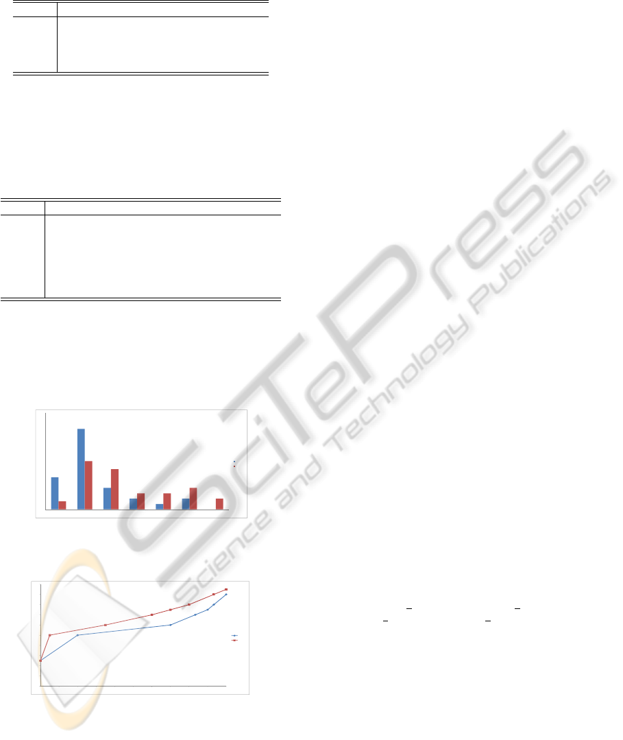
Table 3: Age range and distribution of obtained marks for

two classes of students.

Age Marks

Class 1 [10,12] ([5,10[, 0.2;[10,12[, 0.5;

[12,15[, 0.2;[15,18], 0.1)

Class 2 [11,14] ([5, 10[,0.05;[10, 12[,0.3;[12, 14[, 0.25;

[14,16[, 0.2;[16,19], 0.2;)

In Table 4, the values of the histogram-valued variable

“Marks” are re-written on the intersection partitons.

Table 4: Age range and distribution of obtained marks for

two classes of students, after re-writing the histograms with

the intersection partitions.

Age Marks

Class 1 ([10,11[,0.5; ([5,10[,0.2; [10,12[,0.5; [12,14[,0.133;

[11,12[, 0.5; [14,15[, 0.067;[15,16[, 0.033;

[12,14], 0.0) [16,18[, 0.067;[18,19], 0.0)

Class 2 ([10,11[, 0; ([5,10[,0.05; [10,12[,0.3; [12, 14[,0.25;

[11,12[, 0.33; [14,15[, 0.1;[15,16[, 0.1;

[12,14], 0.67) [16,18[, 0.133;[18,19], 0.067)

Figure 1 represents the the observed histograms of

variable “Marks” for Class 1 and Class 2. Figure 2 de-

picts the respective quantile functions, obtained after

re-writing the histograms with the same partition.

0,1

0,2

0,3

0,4

0,5

0,6

[5,10[ [10,12[ [12,14[ [14,15[ [15,16[ [16,18[ [18,19[

Class 1

Class 2

Figure 1: Representation of Marks(Class 1) and

Marks(Class 2) in the form of histograms.

0 0,1 0,2 0,3 0,4 0,5 0,6 0,7 0,8 0,9 1

Class 1

Class 2

Figure 2: Representation of Marks(Class 1) and

Marks(Class 2) by the quantile functions.

Henceforth “distribution” refers to a probability or

frequency distribution of a continuous variable rep-

resented by a histogram or a quantile function.

3 DIVISIVE CLUSTERING

Divisive clustering algorithms proceed top-down,

starting with Ω, the set to be clustered, and perform-

ing a bipartition of one cluster at each step. At step m

a partition of Ω in m clusters is present, one of which

will be further divided in two sub-clusters; the clus-

ter to be divided and the splitting rule are chosen so

as to obtain a partition in m + 1 clusters minimizing

intra-cluster dispersion.

3.1 The Criterion

The “quality” of a given partition P

(m)

,...,C

(m)

is measured by a crite-

rion Q(m), the sum of intra-cluster dispersion for

each cluster :

Q(m) =

∑

α=1

I(C

) =

∑

α=1

∑

,ω

∈C

(m)

(ω

,ω

) (2)

with D

(ω

,ω

) =

∑

j=1

i j

) (3)

where d is a quadratic distance between distributions

(notice that both for interval-valued and histogram-

valued variables, x

i j

is represented as a distribution).

That is, for each cluster, intra-cluster dispersion is de-

ﬁned as the sum D

of all pairwise squared-distances

between the cluster elements. We consider distances

additive on the descriptive variables.

At each step one cluster is chosen to be split in two

sub-clusters, so that Q(m+1) is minimized, or, equiv-

alently, Q(m) − Q(m + 1) maximized (notice that Q

always decreases at each step).

3.1.1 Distances

Several distances may be considered to evaluate the

dissimilarity between distributions. Let Y

(ω

) =

(ω

)

= ([I

i j1

[, p

i j1

;...;[I

i jK

], p

i jK

). We

propose to use one of the two following distances:

1. Mallows Distance.

i j

) =

i j

(t) − q

(t))

i j

is the quantile function corresponding to the

distribution Y

(ω

2. Squared Euclidean Distance.

i j

) =

∑

`=1

i j`

− p

)

The Mallows distance has been used in agglomerative

hierarchical clustering in (Irpino and Verde, 2006).

ICPRAM 2012 - International Conference on Pattern Recognition Applications and Methods

232

3.2 Binary Questions and Assignment

The bipartition to be performed at each step is deﬁned

by one single variable, considering conditions of the

type R

:= Y

≤ I

,` = 1, . . . , K

− 1, j = 1,..., p,

i.e., we consider the upper bounds I

of all sub-

intervals (except for the last one) corresponding to

each variable.

Each condition R

leads to a bipartition of a clus-

ter, sub-cluster 1 gathers the elements who verify the

condition, sub-cluster 2 those who do not. An ele-

ment ω

∈ Ω veriﬁes the condition R

= Y

≤ I

iff

∑

α=1

i jα

≥ 0.5 (Chavent, 2000).

Notice that the sequence of conditions met by the

elements of each cluster constitutes a necessary and

sufﬁcient condition for cluster membership. The ob-

tained clustering is therefore monothetic, i.e. each

cluster is represented by a conjunction of properties

in the descriptive variables.

Example 3. Consider again the data in Example 2.

At the ﬁrst step, the binary questions to be considered

are :

Age ≤ 11, Age ≤ 12, Marks ≤ 10, Marks ≤ 12, Marks

≤ 14, Marks ≤ 15, Marks ≤ 16, Marks ≤ 18.

If condition Age ≤ 12 is selected, then sub-cluster 1

shall contain Class 1, and be described by “Age ≤

12”, and sub-cluster 2 shall contain Class 2 and be

described by “Age > 12”.

At each step, the cluster C

(m)

and the splitting con-

dition R

are chosen so that the resultant partition

m+1

, in m + 1 clusters) minimizes Q(m + 1).

3.3 The Algorithm

The proposed divisive clustering algorithm may now

be summarized as follows. Let P

= {C

(m)

,...,C

(m)

}

be the current partition at step m.

Initialization : P

= {C

(1)

≡ Ω}. At step m: Deter-

mine the cluster C

(m)

and the binary question R

≤ I

,` = 1, . . . , K

, j = 1, . . . , p, such that the new

resulting partition P

m+1

= {C

(m+1)

,...,C

(m+1)

m+1

}, in

m + 1 clusters, minimizes intra-cluster dispersion,

given by Q(m) =

∑

`=1

∑

,ω

∈C

(m)

∑

j=1

i j

)),

among partitions in m + 1 clusters obtained by split-

ting a cluster of P

in two clusters. Notice that

to minimize Q(m) is equivalent to maximize ∆Q =

I(C

(m)

) − (I(C

(m+1)

) + I(C

(m+1)

)).

When the desired, pre-ﬁxed, number of clusters is

attained, or P has n clusters, each with a single ele-

ment (step n), the algorithm stops.

4 ILLUSTRATIVE EXAMPLE

Table 5 gathers information about the Price (in thou-

sands of dollars) and Engine Displacement (in cm

) of

four utilitarian cars’ models, considering histograms,

already written with the same partitions.

Table 5: Price and Engine Displacement of 4 car models.

Price Engine Displacement

Model 1 ([15, 25[, 0.5;[25,35[, 0.5); ([1300, 1500[,0.2;[1500, 1700[,0.5;

[1700,1900[, 0.3)

Model 2 ([15, 25[, 0.2;[25,35[, 0.8); ([1300, 1500[,0.1;[1500, 1700[,0.2;

[1700,1900[, 0.7)

Model 3 ([15,25[, 0,33;[25, 35[,0.67) ([1300,1500[, 0.1;[1500,1700[, 0.4;

[1700,1900[, 0.5)

Model 4 ([15, 25[,0.6;[25, 35[,0.4) ([1300, 1500[,0.6;[1500, 1700[,0.4;

[1700,1900[, 0.0)

A partition into three clusters is desired. We

choose to use the squared Euclidean distance between

distributions to compare the observed values for each

car model. The distance matrice is then

D =







0.0000 0.4400 0.1178 0.2800

0.4400 0.0000 0.1380 1.1000

0.1178 0.1380 0.0000 0.8429

0.2800 1.1000 0.8429 0.0000







We start with the trivial parti-

tion (in one cluster) P

= {Ω =

{Model 1 , Model 2 , Model 3 , Model 4}}. At step

2, Ω is split into clusters C

(2)

= {Model 1, Model 4}

and C

(2)

= {Model 2, Model 3}, according to condi-

tion R

:= Price ≤ 25; partition P

= {C

(2)

}

has total intra-cluster dispersion equal to 0.3938. At

step 3, C

(2)

is further divided into C

(3)

= { Model 4 }

and C

(

= { Model 1 }, according to condition

:= Engine Displacement ≤ 1500. A partition

in three clusters P

= {C

(3)

= C

(2)

} =

{{Model 4},{Model 1},{Model 2, Model 3}} is

obtained, with intra-cluster dispersion equal to

0.1132. Cluster C

(3)

= {Model 4} is described

by “Price ≤ 25 ∧ Engine Displacement ≤ 1500”;

Cluster C

(3)

= {Model 1} by “Price ≤

25 ∧ Engine Displacement > 1500”; Cluster

(3)

= {Model 2, Model 3} by “Price > 25”.

5 CONCLUSIONS

We have proposed a divisive clustering method for

data described by interval and/or histogram-valued

variables. The method provides a hierarchy on the

DIVISIVE MONOTHETIC CLUSTERING FOR INTERVAL AND HISTOGRAM-VALUED DATA

233

set under analysis, together with a conjunctive char-

acterization of each cluster. Distances for comparing

distributions are considered. Experiments with real-

data allowing for comparision with alternative meth-

ods are planned.

The following step should consist of implementing

a procedure for revising the condition inducing the

cluster chosen for splitting at each step, so as to im-

prove the obtained clustering (in the same line as in

(Chavent, 1998)). Also, the hierarchy may be in-

dexed, so that a dendrogram is obtained. Finally, the

complexity of the computation of the intra-cluster dis-

persion may be reduced by taking into account the or-

der between the cut values I

. These developments

will be the subject of our further research.

REFERENCES

Billard, L. and Diday, E. (2006). Symbolic Data Analysis:

Conceptual Statistics and Data Mining. Wiley.

Bock, H.-H. and Diday, E. (2000). Analysis of Symbolic

Data. Springer, Berlin-Heidelberg.

Boley, D. L. (1998). Principal direction divisive parti-

tioning. Data Mining and Knowledge Discovery,

2(4):325–344.

Breiman, L., Friedman, J. H., Olshen, R. A., and Stone,

C. J. (1984). Classiﬁcation and Regression Trees.

Wadsworth, Belmont, CA.

Brito, P. (1994). Use of pyramids in symbolic data analysis.

In Diday, E. et al., editors, New Approaches in Clas-

siﬁcation and Data Analysis, pages 378–386, Berlin-

Heidelberg. Springer.

Brito, P. (1995). Symbolic objects: order structure and

pyramidal clustering. Annals of Operations Research,

55:277–297.

Brito, P. (1998). Symbolic clustering of probabilistic

data. In Rizzi, A. et al., editors, Advances in Data

Science and Classiﬁcation, pages 385–389, Berlin-

Heidelberg. Springer.

Chavent, M. (1998). A monothetic clustering method. Pat-

tern Recognition Letters, 19(11):989–996.

Chavent, M. (2000). Criterion-based divisive clustering

for symbolic objects. In Bock, H.-H. and Diday, E.,

editors, Analysis of Symbolic Data, pages 299–311,

Berlin-Heidelberg. Springer.

Chavent, M., De Carvalho, F. A. T., Lechevallier, Y., and

Verde, R. (2006). New clustering methods for interval

data. Computational Statistics, 21(2):211–229.

Chavent, M., Lechevallier, Y., and Briant, O. (2007).

DIVCLUS-T: A monothetic divisive hierarchical

clustering method. CSDA, 52(2):687–701.

Ciampi, A. (1994). Classiﬁcation and discrimination: the

RECPAM approach. In Dutter, R. and Grossmann, W.,

editors, Proc. COMPSTAT’94, pages 129–147. Phys-

ica Verlag.

De Carvalho, F. A. T., Brito, P., and Bock, H.-H. (2006).

Dynamic clustering for interval data based on L

dis-

tance. Computational Statistics, 21(2):231–250.

De Carvalho, F. A. T., Csernel, M., and Lechevallier, Y.

(2009). Clustering constrained symbolic data. Pattern

Recognition Letters, 30(11):1037–1045.

De Carvalho, F. A. T. and De Souza, R. M. C. R. (2010).

Unsupervised pattern recognition models for mixed

feature-type symbolic data. Pattern Recognition Let-

ters, 31(5):430–443.

De Souza, R. M. C. R. and De Carvalho, F. A. T. (2004).

Clustering of interval data based on city-block dis-

tances. Pattern Recognition Letters, 25(3):353–365.

Dhillon, I. S., Mallela, S., and Kumar, R. (2003). A divisive

information-theoretic feature clustering algorithm for

text classiﬁcation. Journal of Machine Learning Re-

search, 3:1265–1287.

Diday, E. and Noirhomme-Fraiture, M. (2008). Symbolic

Data Analysis and the Sodas Software. Wiley.

Fang, H. and Saad, Y. (2008). Farthest centroids divisive

clustering. In Proc. ICMLA, pages 232–238.

Gowda, K. C. and Krishna, G. (1978). Disaggregative clus-

tering using the concept of mutual nearest neighbor-

hood. IEEE Trans. SMC, 8:888–895.

Hardy, A. and Baune, J. (2007). Clustering and validation of

interval data. In Brito, P. et al., editors, Selected Con-

tributions in Data Analysis and Classiﬁcation, pages

69–82, Heidelberg. Springer.

Hardy, A. and Kasaro, N. (2009). A new clustering method

for interval data. MSH/MSS, 187:79–91.

Irpino, A. and Verde, R. (2006). A new Wasserstein based

distance for the hierarchical clustering of histogram

symbolic data. In Batagelj, V. et al., editors, Proc.

IFCS 2006, pages 185–192, Heidelberg. Springer.

Kaufman, L. and Rousseeuw, P. J. (1990). Finding Groups

in Data. Wiley, New York.

Lance, G. N. and Williams, W. T. (1968). Note on a new

information statistic classiﬁcation program. The Com-

puter Journal, 11:195–197.

MacNaughton-Smith, P. (1964). Dissimilarity analysis: A

new technique of hierarchical subdivision. Nature,

202:1034–1035.

Michalski, R. S., Diday, E., and Stepp, R. (1981). A

recent advance in data analysis: Clustering objects

into classes characterized by conjunctive concepts. In

Kanal, L. N. and Rosenfeld, A., editors, Progress in

Pattern Recognition, pages 33–56. Springer.

Michalski, R. S. and Stepp, R. (1983). Learning from ob-

servations: Conceptual clustering. In Michalsky, R. S.

et al., editors, Machine Learning: An Artiﬁcial Intelli-

gence Approach, pages 163–190. Morgan Kaufmann.

Noirhomme-Fraiture, M. and Brito, P. (2011). Far beyond

the classical data models: Symbolic data analysis. Sta-

tistical Analysis and Data Mining, 4(2):157–170.

Quinlan, J. R. (1986). Induction of decision trees. Machine

Learning, 1:81–106.

Sneath, P. H. and Sokal, R. R. (1973). Numerical Taxonomy.

Freeman, San Francisco.

Williams, W. T. and Lambert, J. M. (1959). Multivariate

methods in plant ecology. J. Ecology, 47:83–101.

ICPRAM 2012 - International Conference on Pattern Recognition Applications and Methods

234