CLASSIFICATION USING HIGH ORDER DISSIMILARITIES
IN NON-EUCLIDEAN SPACES
Helena Aidos
1
, Ana Fred
1
and Robert P. W. Duin
2
1
Instituto de Telecomunicac¸˜oes, Instituto Superior T´ecnico, Lisbon, Portugal
2
Faculty of Electrical Engineering, Mathematics and Computer Sciences, Delft University of Technology,
Delft, The Netherlands
Keywords:
Dissimilarity increments, Maximum a posteriori, Classification, Gaussian mixture, Non-Euclidean space.
Abstract:
This paper introduces a novel classification algorithm named MAP-DID. This algorithm combines a maximum
a posteriori (MAP) approach using the well-known Gaussian Mixture Model (GMM) method with a term that
forces the various Gaussian components within each class to have a common structure. That structure is
based on higher-order statistics of the data, through the use of the dissimilarity increments distribution (DID),
which contains information regarding the triplets of neighbor points in the data, as opposed to typical pairwise
measures, such as the Euclidean distance. We study the performance of MAP-DID on several synthetic and real
datasets and on various non-Euclidean spaces. The results show that MAP-DID outperforms other classifiers
and is therefore appropriate for classification of data on such spaces.
1 INTRODUCTION
Classification deals with algorithmic methodologies
for assigning a new input data to one of the known
classes. There are numerous classifiers with differ-
ent strategies, like k nearest neighbor, neural net-
works, support vector machines, Parzen windows
(Duda et al., 2001; Hastie et al., 2009).
This paper introduces a new maximum a posteri-
ori (MAP) classifier based on the Gaussian Mixture
Model (GMM). This novel classifier (MAP-DID) in-
troduces an extra factor on the likelihood containing
information about higher-order statistics of the data,
through the use of the distribution of their dissimilar-
ity increments (Aidos and Fred, 2011).
2 DISSIMILARITY
REPRESENTATIONS
Sometimes it is useful to describe the objects using a
dissimilarity representation, a square matrix contain-
ing the dissimilarities between all pairs of objects. To
use the typical classifiers, we need to build a vector
space based on the relations given by the dissimilar-
ity matrix. In (Duin and Pekalska, 2008), two strate-
gies are considered to obtain vector spaces: pseudo-
Euclidean spaces and dissimilarity spaces.
2.1 Pseudo-Euclidean Spaces (PES)
The PES is given by the Cartesian product of two
real spaces: E = R
p
×R
q
. A vector x ∈ E is rep-
resented as an ordered pair of two real vectors: x =
(x
+
,x
−
). This space is equipped with a pseudo-inner
product, such that hx, yi
E
= x
T
J
pq
y, where J
pq
=
[I
p×p
0;0 −I
q×q
]. Alternatively, if x
+
i
and x
−
i
rep-
resent the components of x
+
and x
−
, then hx,yi
E
=
∑
p
i=1
x
+
i
y
+
i
−
∑
q
i=1
x
−
i
y
−
i
.
Although this pseudo-inner product is symmetric
and linear in its first argument, it is not positive defi-
nite. Thus, if one constructs the Gram matrix, G, from
the data patterns x
i
as G
ij
= x
T
i
x
j
, then G may not be
positive semidefinite in the PES (Pekalska, 2005). G
is symmetric in the PES, so it has an eigendecompo-
sition of G = VDV
T
; but, its eigenvalues can be neg-
ative. Note that a new dataset can be built up from
G through X = V|D|
1/2
, where matrix X contains the
vector representations of the new patterns in the PES.
In (Duin et al., 2008; Duin and Pekalska, 2008),
several variants of PES are considered. In this paper,
we also consider the following spaces.
• Pseudo-Euclidean Space (PES): This is a (p +
q)-dimensional PES defined by p + q eigenvec-
tors. One keeps the p largest positive eigenvalues
306
Aidos H., Fred A. and P. W. Duin R. (2012).
CLASSIFICATION USING HIGH ORDER DISSIMILARITIES IN NON-EUCLIDEAN SPACES.
In Proceedings of the 1st International Conference on Pattern Recognition Applications and Methods, pages 306-309
DOI: 10.5220/0003779503060309
Copyright
c
 SciTePress

and the q negative eigenvalues that have the high-
est absolute value. Each direction is scaled by the
magnitude of the corresponding eigenvalue.
• Positive Pseudo-Euclidean Space (PPES): This
p-dimensional space is defined as PES, but only
the p largest positive eigenvalues are kept.
• Negative Pseudo-Euclidean Space (NPES): This
q-dimensional space is defined as PES, but only
the q largest negative eigenvalues (in magnitude)
are kept; no positive eigenvalues are used.
• Corrected Euclidean Space (CES): In CES, a
constant is added to all the eigenvalues (positive
and negative) to ensure that they all become pos-
itive. This constant is given by 2|a|, where a is
the negative eigenvalue with the largest absolute
value.
2.2 Dissimilarity Spaces (DS)
We consider four more spaces constructed in the fol-
lowing way: we compute the pairwise Euclidean dis-
tances between data points of one of the spaces de-
fined above. These distances are new feature repre-
sentations of x
i
. Note that the dimension of the fea-
ture space is equal to the number of points.
Since our classifier suffers from the curse of di-
mensionality, we must reduce the number of features;
there are several techniques for that (Hastie et al.,
2009). We chose k-means to find a number of pro-
totypes k < N. k is selected as a certain percent-
age of N/2, and the algorithm is initialized in a de-
terministic way as described in (Su and Dy, 2007).
After the k prototypes are found, the distances from
each point x
i
to each of these prototypes are used
as their new feature representations. This defines
four new spaces, which are named as Dissimilarity
Pseudo-Euclidean Space (DPES), Dissimilarity Posi-
tive Pseudo-Euclidean Space (DPPES), Dissimilarity
Negative Pseudo-Euclidean Space (DNPES) and Dis-
similarity Corrected Euclidean Space (DCES).
3 THE MAP-DID ALGORITHM
In this section, dissimilarities between patterns in the
eight previously defined spaces are computed as Eu-
clidean distances.
3.1 Dissimilarity Increments
Distribution (DID)
Let X be a set of patterns, and (x
i
,x
j
,x
k
) a triplet
of nearest neighbors belonging to X, where x
j
is the
nearest neighbor of x
i
and x
k
is the nearest neighbor
of x
j
, different from x
i
. The dissimilarity increment
(DI) (Fred and Leit˜ao, 2003) between these patterns
is defined as d
inc
(x
i
,x
j
,x
k
) =


d(x
i
,x
j
) −d(x
j
,x
k
)


.
This measure contains information different from a
distance: the latter is a pairwise measure, while the
former is a measure for a triplet of points, thus a mea-
sure of higher-order dissimilarity of the data.
In (Aidos and Fred, 2011) the DIs distribution
(DID) was derived under the hypothesis of Gaussian
distribution of the data and it was written as a function
of the mean value of the DIs, λ. Therefore, the DID
of a class is given by
p
d
inc
(w;λ) =
πβ
2
4λ
2
wexp

−
πβ
2
4λ
2
w
2

+
π
2
β
3
8
√
2λ
3
×

4λ
2
πβ
2
−w
2

exp

−
πβ
2
8λ
2
w
2

erfc

√
πβ
2
√
2λ
w

, (1)
where erfc(·) is the complementary error function,
and β = 2−
√
2.
3.2 MAP-DID
Consider that {x
i
,c
i
,inc
i
}
N
i=1
is our dataset, where x
i
is a feature vector in R
d
, c
i
is the class label and inc
i
is the set of increments yielded by all the triplets of
points containing x
i
. We assume that a class c
i
has
a single statistical model for the increments, with an
associated parameter λ
i
. This DID, described above,
can be seen as high-order statistics of the data since it
has information of a third order dissimilarity of data.
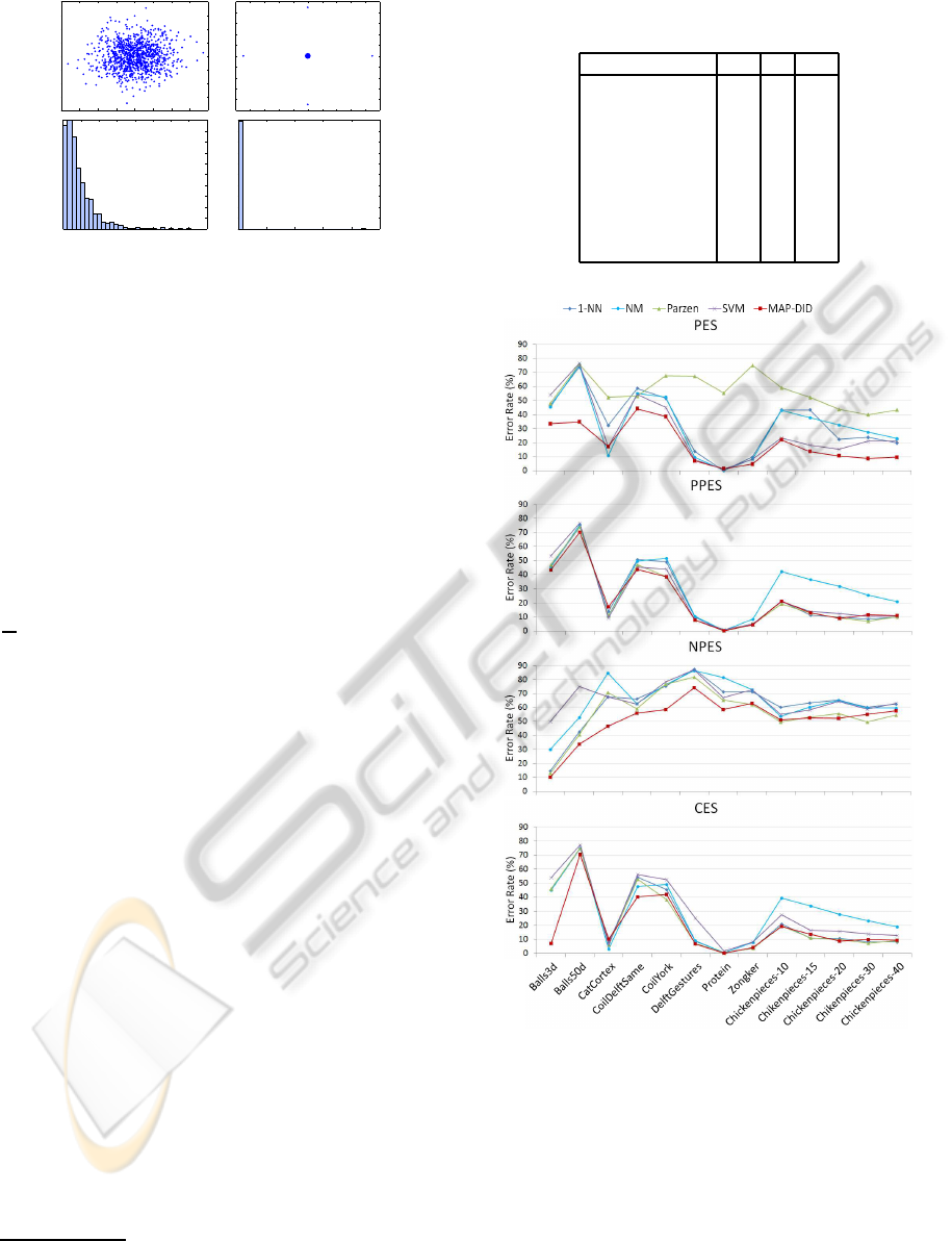
For example, we generate a 2-dimensional Gaus-
sian with 1000 points; it has zero mean and covari-
ance the identity matrix (figure 1 left). We also
generate a 2-dimensional dataset with 1000 points,
where 996 points are in the center and there are four
off-center points at coordinates (±a, 0) and (0,±a),
where a is such that the covariance is also the identity
matrix (figure 1 right). We compute the DIs for each
dataset and look at their histograms (figure 1).
Although the datasets have the same mean and co-
variancematrix, the two DIs distributionsare very dif-
ferent from each other. Therefore, the DIs can be seen
as a measure of higher-order statistics: the two dis-
tributions under consideration have exactly the same
mean and variance, but their DIDs are vastly different.
So, we design a maximum a posteriori (MAP)
classifier that combines the Gaussian Mixture Model
(GMM) and the information given by the increments,
assuming that x
i
and inc
i
are conditionally indepen-
dent given c
j
. We used a prior given by p(c
j
) =
|c
j
|/N, with |c
j
| the number of points of class j, and
the likelihood p(x
i
,inc
i
|c
j
) = p(x
i
|c
j
)p(inc
i
|c
j
).
CLASSIFICATION USING HIGH ORDER DISSIMILARITIES IN NON-EUCLIDEAN SPACES
307

−25 −20 −15 −10 −5 0 5 10 15 20 25
−25
−20
−15
−10
−5
0
5
10
15
20
25
0 0.05 0.1 0.15 0.2 0.25 0.3 0.35 0.4
0
20
40
60
80
100
120
140
160
180
200
0 5 10 15 20 25
0
100
200
300
400
500
600
700
800
900
1000
−4 −3 −2 −1 0 1 2 3 4
−4
−3
−2
−1
0
1
2
3
4
Figure 1: Two simple datasets with zero mean and a covari-
ance given by the identity matrix, but with vastly different
DIs. Left: Gaussian data. Right: dataset with 996 points
at the origin and four off-center points. Corresponding his-
tograms of the DIs. Note that in the right histogram there
are four non-zero increments and 996 zero increments.
The class-conditional density of the vector x
i
fol-
lows a GMM given by p(x
i
|c
j
) =
∑
K
l=1
α
l
p(x
i
|Σ
l
,µ
l
),
with K the number of Gaussian components deter-
mined for class c
j
, α
l
the weight of each Gaussian
component and p(x
i
|Σ
l
,µ
l
) the Gaussian distribution.
We obtained the parameters α
l
, Σ
l
and µ
l
using the
GMM described in (Figueiredo and Jain, 2002).
The class-conditional density of the set of in-
crements where x
i
belongs is given by p(inc
i
|c
j
) =
1
M
∑
M
n=1
p(inc
n
i
|c
j
), where M is the number of incre-
ments of the set inc
i
, inc
n
i
is the n-th increment of that
set, and p(inc
i
|c
j
) = p(inc
i
|λ
j
) is the DID given in
equation (1). We thus consider a statistical model for
increments with parameter λ
j
for each class.
4 EXPERIMENTAL RESULTS
AND DISCUSSION
In this section we compare MAP-DID to other classi-
fiers (1-nearest neighbor (1-NN), nearest-mean (NM),
Parzen window and a linear support vector machine
(SVM)). We use 13 datasets, of which 2 are synthetic
and 11 are real-world data
1
.
For each of the classifiers, we use a 10-fold cross-
validation scheme to estimate classifier performance.
Figures 2 and 3 present the results for the average
classification error. The values of p and q eigenvec-
tors, and k prototypes, used to construct the spaces
described in Section 2, are in Table 1.
The MAP-DID is the algorithm with the lowest
error rate. This is true for the vast majority of all
the possible dataset-space pairs. Thus, if any of these
1
See http://prtools.org/disdatasets/ for a full description
of the datasets and the MATLAB toolboxes containing the
classifiers used for comparison.
Table 1: Number of eigenvectors and prototypes used to
construct the spaces described in Section 2.
Dataset p q k
Balls3d 3 7 10
Balls50d 18 5 18
CatCortex 2 2 2
CoilDelftSame 8 4 7
CoilYork 8 5 7
DelftGestures 11 2 13
Protein 6 2 5
Zongker 14 3 20
Chickenpieces 8 3 9
Figure 2: Classification error rate on the four pseudo-
Euclidean spaces considered in Section 2.1.
spaces are to be used for classification, the MAP-DID
is a good choice for classification algorithm.
Some other interesting points should be empha-
sized: for the real-world datasets it is interesting to
note that the results are not very different between the
PES, PPES and CES spaces, all of which take into ac-
count the positive portion of the space. Conversely,
the NPES results are considerably worse than those
ICPRAM 2012 - International Conference on Pattern Recognition Applications and Methods
308

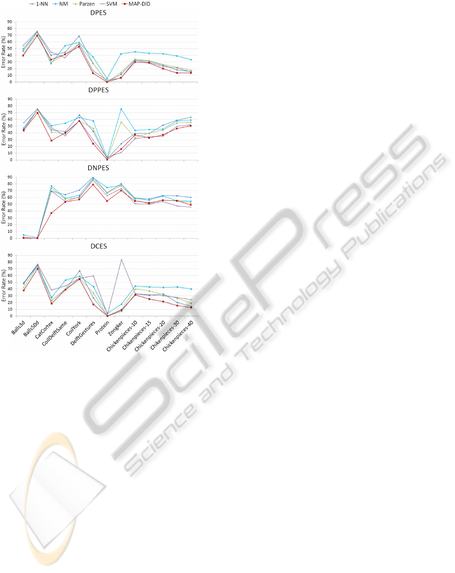
Figure 3: Classification error rate on the four dissimilarity
spaces considered in Section 2.2.
three, which indicates that this negative space con-
tains little information for classification purposes.
Another interesting point is that in the dissimilar-
ity spaces (figure 3), neither the positive (DPPES) nor
the negative (DNPES) spaces contain all the informa-
tion; instead, the union of the information contained
in those two spaces (DPES or DCES) yields much
better results than either of them separately.
It was necessary to reduce the dimensionality of
the data to generate the dissimilarity spaces (figure 3).
This reduction was accomplished through k-means,
by computing the distances from the data patterns to
the estimated prototypes. However, many other tech-
niques could be used for dimensionality reduction,
and it is possible that some of those techniques would
yield an improvement on the results for these spaces.
One aspect not considered here is the metric-
ity and euclideaness of datasets (Duin and Pekalska,
2008). These properties may help us identify the sit-
uations where MAP-DID performs well.
5 CONCLUSIONS
We have presented a novel maximum a posteriori
(MAP) classifier which uses the dissimilarity incre-
ments distribution (DID). This classifier, called MAP-
DID, can be interpreted as a Gaussian Mixture Model
with an operator that forces a class to have a com-
mon increment structure, even though each Gaussian
component within a class can have distinct means and
covariances. Experimental results have shown that
MAP-DID outperforms multiple other classifiers on
various datasets and feature spaces.
In this paper we focused on Euclidean spaces de-
rived from non-Euclidean data. This might suggest
that MAP-DID could perform well when applied to
originally Euclidean data. This is a topic which will
receive more investigation in the future.
ACKNOWLEDGEMENTS
This work was supported by the FET programme
within the EU FP7, under the SIMBAD project con-
tract 213250; and partially by the Portuguese Foun-
dation for Science and Technology, scholarship num-
ber SFRH/BD/39642/2007, and grant PTDC/EIA-
CCO/103230/2008.
REFERENCES
Aidos, H. and Fred, A. (2011). On the distribution of dis-
similarity increments. In IbPRIA, pages 192–199.
Duda, R. O., Hart, P. E., and Stork, D. G. (2001). Pattern
Classification. John Wiley & Sons Inc., 2nd edition.
Duin, R., Pekalska, E., Harol, A., Lee, W.-J., and Bunke, H.
(2008). On euclidean corrections for non-euclidean
dissimilarities. In SSPR/SPR, pages 551–561.
Duin, R. P. and Pekalska, E. (2008). On refining dissimilar-
ity matrices for an improved nn learning. In ICPR.
Figueiredo, M. and Jain, A. (2002). Unsupervised learn-
ing of finite mixture models. IEEE Trans. on Pattern
Analysis and Machine Intelligence, 24(3):381–396.
Fred, A. and Leit˜ao, J. (2003). A new cluster isolation
criterion based on dissimilarity increments. IEEE
Trans. on Pattern Analysis and Machine Intelligence,
25(8):944–958.
Hastie, T., Tibshirani, R., and Friedman, J. (2009). The Ele-
ments of Statistical Learning: Data Mining, Inference,
and Prediction. Springer, 2nd edition.
Pekalska, E. (2005). Dissimilarity Representations in Pat-
tern Recognition: Concepts, Theory and Applications.
PhD thesis, Delft University of Technology, Delft,
Netherland.
Su, T. and Dy, J. G. (2007). In search of deterministic
methods for initializing k-means and gaussian mixture
clustering. Intelligent Data Analysis, 11(4):319–338.
CLASSIFICATION USING HIGH ORDER DISSIMILARITIES IN NON-EUCLIDEAN SPACES
309