SCALE-INDEPENDENT SPATIO-TEMPORAL STATISTICAL SHAPE

REPRESENTATIONS FOR 3D HUMAN ACTION RECOGNITION

Marco K

orner, Daniel Haase and Joachim Denzler

Department of Mathematics and Computer Sciences, Friedrich Schiller University of Jena

Ernst-Abbe-Platz 2, 07743 Jena, Germany

Keywords:

Human action recognition, Manifold learning, PCA, Shape model.

Abstract:

Since depth measuring devices for real-world scenarios became available in the recent past, the use of 3d data

now comes more in focus of human action recognition. We propose a scheme for representing human actions in

3d, which is designed to be invariant with respect to the actor’s scale, rotation, and translation. Our approach

employs Principal Component Analysis (PCA) as an exemplary technique from the domain of manifold learning.

To distinguish actions regarding their execution speed, we include temporal information into our modeling

scheme. Experiments performed on the CMU Motion Capture dataset shows promising recognition rates as

well as its robustness with respect to noise and incorrect detection of landmarks.

1 INTRODUCTION AND

RELATED WORK

In the last decades the recognition and analysis of ac-

tions and motions performed by humans have become

one of the most promising ﬁelds in computer vision

research and lead to a wide variety for research top-

ics in computer vision. This family of problems aims

to determine human activities automatically based on

several sensor observations. A wide range of indus-

trial as well as academic applications are based on this

research, e. g. the interaction between humans and ma-

chines, surveillance and security, entertainment, video

content retrieval as well as the research in medical and

life sciences.

In early years of scientiﬁc interest those methods

concentrated on the evaluation of 2d image sequences

delivered by gray value or color cameras (Gavrila,

1999; Turaga et al., 2008; Poppe, 2010). Due to

the massive amount of research those methods now

achieve very good results on the standard Weizmann

2d action recognition dataset (Gorelick et al., 2007).

Several of those approaches are based on the evalua-

tion of changes in silhouettes or the extraction of in-

terest point features in space-time volumes created by

subsequent video frames (Laptev, 2005; Dollar et al.,

2005). Furthermore the combination of shape and

optical ﬂow is used for action recognition (Ke et al.,

2007).

In contrast to this huge amount of scientiﬁc work

concerning 2d images, 3d data was not yet used in a

remarkable quantity. However, the recent development

of depth measuring devices such as Time-of-Flight

(ToF) sensors or sensors based on the projection and

capturing of structured light patterns make 3d data

available in a fast and inexpensive way.

In this paper we present a spatio-temporal represen-

tation scheme for human actions given as sequences

of 3d landmark positions which models the spatial

variations in a contextual way and takes into account

the temporal coherence between subsequent frames

based on manifold learning techniques. After present-

ing our approach in Sec. 2 we show numerous experi-

ments evaluated on the CMU Motion Capture (MoCap)

dataset in Sec. 3. A summary and a brief outlook in

Sec. 4 conclude this paper.

2 STATISTICAL SHAPE

REPRESENTATION

Manifold learning techniques are widely used for

classiﬁcation tasks like face detection and emotion

recognition (Zhang et al., 2005). For action recogni-

tion from 2d video streams the usability of Principle

Component Analysis (PCA), and Independent Compo-

nent Analysis (ICA) on motion silhouettes have been

compared (Yamazaki et al., 2007). Locality Preserv-

ing Projections (LPP) were utilized in combination

with a special Hausdorff distance measure on silhou-

ettes (Wang and Suter, 2007). A comparison of further

techniques for dimensionality reduction like Locality

Sensitive Discriminative Analysis (LSDA) and Local

288

Körner M., Haase D. and Denzler J. (2012).

SCALE-INDEPENDENT SPATIO-TEMPORAL STATISTICAL SHAPE REPRESENTATIONS FOR 3D HUMAN ACTION RECOGNITION.

In Proceedings of the 1st International Conference on Pattern Recognition Applications and Methods, pages 288-294

DOI: 10.5220/0003766202880294

 SciTePress

(a) (b)

Figure 1: (a) The skeleton model used in our approach with

31 joints affected by 62 degrees of freedom. (b) Data matrix

for action class

walking

indicating the sequential parameter

changes. The colors of the columns are corresponding to

the colors in the model while the intensities illustrate the

parameter values.

Spatio-Temporal Discriminant Embedding (LSTDE)

was presented in (Jia and Yeung, 2008). Tensor PCA

for reducing the dimensionality of the parameter space

was also investigated (Sun et al., 2011).

In the ﬁeld of 3d action recognition far less work

exist. Laplacian Eigenmaps are recently used to rec-

ognize human actions from 3d points delivered by

full-body ToF scans (Schwarz et al., 2010; Schwarz

et al., 2012). Hierarchical Gaussian Process La-

tent Variable Modeling (H-GPLVM) combined with

Conditional Random Fields (CRF) was employed to

model relations between limbs action classiﬁcation

from CMU MoCap data (Han et al., 2010).

For action recognition in 3d data a unique repre-

sentation is necessary, which needs to be invariant

against absolute landmark positions. While Active

Shape Models (ASM) (Cootes et al., 1995) are mas-

sively used in facial expression classiﬁcation, their

main ideas are also suitable for the ﬁeld of locomotion

analysis (Haase and Denzler, 2011).

In the following we use a basic idea of ASMs to

model and recognize human actions in 3d data.

2.1 Spatial Representation

Using a hierarchical skeleton model as shown in

Fig. 1(a), any arbitrary skeleton conﬁguration at time

step

1 ≤ t ≤ N

can be parameterized as a vector of

Euler angles



, . . . , θ



∈ R

while

the number of joint angles. These angles are indi-

cating the rotations of every limb wrt. the adjacent

joints in any room direction limited to its number of

Degrees of Freedom (DoF). E. g. , the neck joint has 3

DoF, because it can rotate in all coordinate directions,

while the elbow has only 2 DoF. The model used in

this paper consists of

= 31

joints which yields 59

DoF and an additional global displacement

(x, y, z)

When using ASMs, normally as a ﬁrst step the land-

−4

−2

−5

−15

−10

−5

−4

−2

−15

−10

−5

−4

−2

−15

−10

−5

(a)

(b)

Figure 2: The ﬁrst three motion components of a

walking

action (a) and their corresponding eigenvectors (b). Colors

indicate the weighting of the eigenvectors added to the mean

shape (

black: w

= −2λ

blue: w

= 0

red: w

= 2λ

Note the anti-symmetric motion directions of the limbs in

the ﬁrst two components and the symmetric one in the third

component.

mark sets have to be aligned in terms of rotation, scale

and translation using Procrustes analysis (Bookstein,

1997). This becomes obsolete in our scenario when

normalizing the actor’s skeleton in an anatomically cor-

rect fashion by setting the root rotation and translation

to θ

= θ

= x

= y

= z

= 0, 1 ≤ t ≤ N

While angular representations tend to be ambigu-

ous because of their periodical nature, joint rotations

are projected to 3d landmark positions

= π

θ→l







(x, y, z)

, . . . , (x, y, z)



∈ R

, (1)

1 ≤ t ≤ N

, using a projection function

θ→l

: R

7→

. To preserve scale invariance of our modeling, a

predeﬁned skeleton model is used for projection each

time.

Combining all zero-mean skeleton conﬁgurations

at every available time step yields the matrix of land-

marks

L =







− l







∈ R

×N

, l

∑

i=1

. (2)

Performing Principle Component Analysis (PCA) on

L will return its matrix

= (v

|···|v

) ∈ R

×N

(3)

of eigenvectors sorted according to their correspond-

ing eigenvalues

descendingly representing the im-

portance of each data space direction. Using these

eigenvectors as basis vectors, every arbitrary skele-

ton conﬁguration represented by a 3d landmark coor-

dinate set can be expressed as a linear combination

= l

+ P

of the data matrix columns and the

frame-speciﬁc shape parameter vector

added to the

constant mean shape l

Since the amount of represented variances of land-

mark sequences captured by the eigenvectors decreases

SCALE-INDEPENDENT SPATIO-TEMPORAL STATISTICAL SHAPE REPRESENTATIONS FOR 3D HUMAN

ACTION RECOGNITION

289

Table 1: Action classes selected from CMU MoCap dataset used in our experiments.

−4

−2

−4

−2

−15

−10

−5

−10

−5

−15

−10

−5

−4

−2

−5

−15

−10

−5

−4

−2

−5

−15

−10

−5

−4

−2

−15

−10

−5

−15

−10

−5

−2

−15

−10

−5

−2

−15

−10

−5

Class walking running marching sneaking hopping jumping golfing salsa

Samples 38 28 14 15 14 9 11 30

Actors 9 9 4 5 4 3 2 2

Avg. frame number 1283 853 6426 4200 602 1325 8626 5224

massively according to the evolution of their corre-

sponding eigenvalues, the number of columns in the

eigenvector matrix

can be restricted to achieve a

substantial reduction of dimensionality.

Fig. 2(a) shows the ﬁrst three action components,

while Fig. 2(b) depicts the corresponding eigenvectors

of an action from class walking.

2.2 Integration of Temporal Context

While the previously described representation solely

models linear variations of skeleton joints, the tempo-

ral evolution of conﬁgurations might contribute helpful

information for the recognition and analysis of articu-

lated actions. For this reason, our model is extended

to include this temporal component.

In (Bosch et al., 2002) such a temporal modeling of

periodical actions was already used to model a beating

heart. This was pointed out to be a generalization of the

multi-view integration approach of (Lelieveldt et al.,

2003) and (Oost et al., 2006). Instead of considering

a skeleton conﬁguration at a single time step

obtain the model parameters, they regard a series of

sequential time steps

< t

< . . . < t

or alternatively

multiple views

, o

, . . . , o

)

at the same time step as

a single conﬁguration.

Applied to our problem, the provided method mod-

els the temporal evolution of skeleton conﬁgurations

by appending subsequent input matrices horizontally:

→t

hist



, l

, ··· , l

hist



∈ R

hist

+1)·N

, (4)

→t

hist







··· l

hist

··· l

hist

−k

hist

−k

hist

)+1

··· l







∈ R

hist

+1)·N

×(N

−(k

hist

+1))

This approach allows us to distinguish between an

action and its reverse counterpart as well as to classify

the speed of execution.

3 EXPERIMENTS

3.1 Dataset

In order to evaluate the proposed methods, we have

chosen eight different actions performed by different

actors from the CMU MoCap dataset, as shown in

more detail in Tab. 1. While we have selected common

actions with slightly different executions like

walking

running

marching

and

sneaking

hopping

and

jumping

, we also took complex motions—

salsa

and

golfswinging—into account.

3.2 Discriminability of Eigenvector

Representation

When performing PCA on sequential data

, the re-

sult shows the most important directions of variance

in the data. For this reason, the eigenvectors

corre-

sponding to the largest eigenvalues

are supposed

to encode most of the information, while the eigen-

vectors corresponding to the lower eigenvalues model

only minor changes in the data as well as noise.

Fig. 3 depicts the evolution of the eigenvalues for

all action classes in our dataset. As can be seen, after a

strong descent up to the third principal component, the

eigenvalues converged strongly towards zero. After

a certain component, there was no substantial contri-

bution to the data, which became apparent at the 12

eigenvalue, as indicated by the vertical line in Fig. 3.

As depicted in Tab. 2, in most the cases two to three

eigenvectors were sufﬁcient to cover

90%

of the vari-

ances occurred while execution of an action. Solely

the action classes with high variances in all directions

need more discriminability, which can be handled by

increasing the number of eigenvectors. This fact can

also be seen in Tab. 3, where the ﬁrst three eigenvectors

are shown together with their mean shapes l

The back projection error

action

) =



· P

action



· P

action

− l

obtained by trans-

ICPRAM 2012 - International Conference on Pattern Recognition Applications and Methods

290

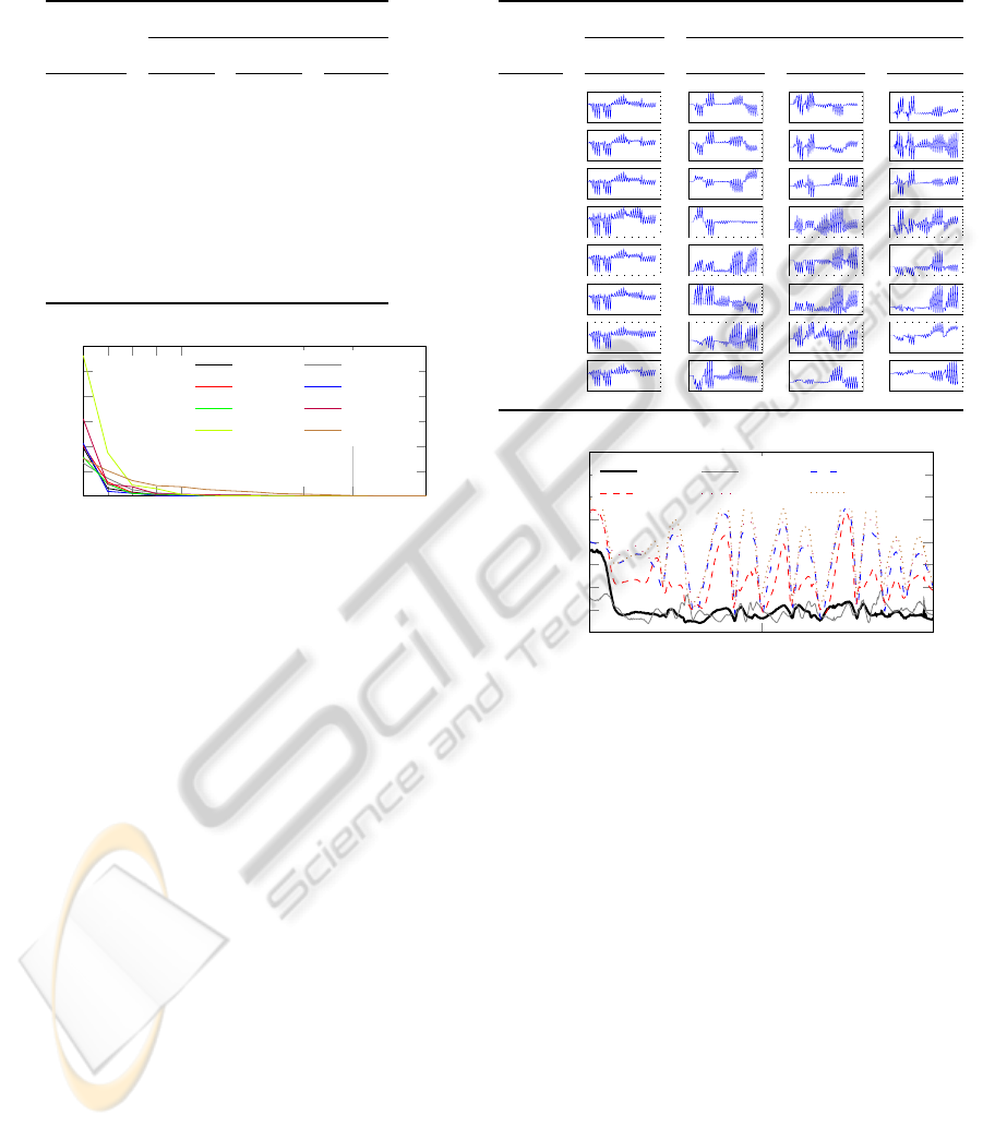
Table 2: Comparison of variance covering facilities of our

representation scheme. While the usage of two to three

eigenvectors allows to achieve 90% of the variances ob-

tained during simple actions, more dimensions are needed

to represent more complex actions.

Action Class Amount of variance

90% 95% 98%

walking 2 3 4

running 2 3 5

marching 3 5 8

sneaking 3 5 8

hopping 2 5 8

jumping 3 4 6

golfing 3 3 4

salsa 8 9 12

1 2 3 4

100

200

300

400

500

600

Principal component k of recorded action

Eigenvalue λ

hopping jumping

running walking

sneaking marching

golfing

salsa

Figure 3: Evolution of eigenvalues for different action

classes. Eigenvalues are decreasing massively up to the

third component, while they remain static for higher-order

components.

forming an arbitrary skeleton conﬁguration

from

Euclidian space

into the reduced eigenspace

action

of a certain action class and back to Euclidian

space, where

action



action



···



action



is a

matrix containing the eigenvectors corresponding

to the ﬁrst

largest eigenvalues of

action

, give a

quantitative justiﬁcation for this postulation, as can be

seen in Fig. 4. As a result, the ordering of remaining

eigenvectors is no longer meaningful. Therefore, they

are not considered in the following classiﬁcation

purposes.

3.3 Feature Vector Design and

Classiﬁcation

In order to distinguish action classes, features have

to be derived from the sequence of skeleton conﬁg-

urations. Using the representation described before,

feature vectors



, v

, . . . , v



are extracted

from a series

of landmark vectors

by concatenat-

ing its mean shape

and its eigenvectors correspond-

Table 3: Comparison of the mean shapes and the ﬁrst three

eigenvectors of the action classes in our dataset. Note that

similar actions have similar ﬁrst eigenvectors and different

second or third eigenvectors while different actions can al-

ready be distinguished by their ﬁrst eigenvectors.

Action

Class

Mean Shape Eigenvectors

walking

0 10 20 30 40 50 60 70 80 90 100

−20

−15

−10

−5

0 10 20 30 40 50 60 70 80 90 100

−0.4

−0.3

−0.2

−0.1

0.1

0.2

0.3

0 10 20 30 40 50 60 70 80 90 100

−0.4

−0.3

−0.2

−0.1

0.1

0.2

0.3

0 10 20 30 40 50 60 70 80 90 100

−0.2

−0.1

0.1

0.2

0.3

0.4

0.5

running

0 10 20 30 40 50 60 70 80 90 100

−20

−15

−10

−5

0 10 20 30 40 50 60 70 80 90 100

−0.4

−0.3

−0.2

−0.1

0.1

0.2

0.3

0 10 20 30 40 50 60 70 80 90 100

−0.3

−0.2

−0.1

0.1

0.2

0.3

0.4

0 10 20 30 40 50 60 70 80 90 100

−0.2

−0.15

−0.1

−0.05

0.05

0.1

0.15

0.2

0.25

marching

0 10 20 30 40 50 60 70 80 90 100

−20

−15

−10

−5

0 10 20 30 40 50 60 70 80 90 100

−0.4

−0.3

−0.2

−0.1

0.1

0.2

0.3

0 10 20 30 40 50 60 70 80 90 100

−0.3

−0.2

−0.1

0.1

0.2

0.3

0.4

0 10 20 30 40 50 60 70 80 90 100

−0.4

−0.3

−0.2

−0.1

0.1

0.2

0.3

0.4

sneaking

0 10 20 30 40 50 60 70 80 90 100

−15

−10

−5

0 10 20 30 40 50 60 70 80 90 100

−0.4

−0.3

−0.2

−0.1

0.1

0.2

0.3

0.4

0 10 20 30 40 50 60 70 80 90 100

−0.1

−0.05

0.05

0.1

0.15

0.2

0.25

0.3

0 10 20 30 40 50 60 70 80 90 100

−0.2

−0.15

−0.1

−0.05

0.05

0.1

0.15

0.2

0.25

0.3

hopping

0 10 20 30 40 50 60 70 80 90 100

−20

−15

−10

−5

0 10 20 30 40 50 60 70 80 90 100

−0.05

0.05

0.1

0.15

0.2

0.25

0.3

0 10 20 30 40 50 60 70 80 90 100

−0.25

−0.2

−0.15

−0.1

−0.05

0.05

0.1

0.15

0.2

0.25

0 10 20 30 40 50 60 70 80 90 100

−0.2

−0.1

0.1

0.2

0.3

0.4

0.5

jumping

0 10 20 30 40 50 60 70 80 90 100

−20

−15

−10

−5

0 10 20 30 40 50 60 70 80 90 100

−0.15

−0.1

−0.05

0.05

0.1

0.15

0.2

0.25

0.3

0 10 20 30 40 50 60 70 80 90 100

−0.05

0.05

0.1

0.15

0.2

0.25

0.3

0.35

0 10 20 30 40 50 60 70 80 90 100

−0.1

−0.05

0.05

0.1

0.15

0.2

0.25

0.3

0.35

golfing

0 10 20 30 40 50 60 70 80 90 100

−20

−15

−10

−5

0 10 20 30 40 50 60 70 80 90 100

−0.2

−0.15

−0.1

−0.05

0.05

0.1

0.15

0.2

0.25

0.3

0 10 20 30 40 50 60 70 80 90 100

−0.2

−0.15

−0.1

−0.05

0.05

0.1

0.15

0.2

0.25

0 10 20 30 40 50 60 70 80 90 100

−0.4

−0.3

−0.2

−0.1

0.1

0.2

0.3

salsa

0 10 20 30 40 50 60 70 80 90 100

−20

−15

−10

−5

0 10 20 30 40 50 60 70 80 90 100

−0.25

−0.2

−0.15

−0.1

−0.05

0.05

0.1

0.15

0.2

0.25

0 10 20 30 40 50 60 70 80 90 100

−0.2

−0.1

0.1

0.2

0.3

0.4

0.5

0 10 20 30 40 50 60 70 80 90 100

−0.4

−0.3

−0.2

−0.1

0.1

0.2

0.3

500

1,000

Frame number

Back projection error ε

action

hopping jumping walking

running sneaking marching

Figure 4: Back projection errors obtained by transforming

skeleton conﬁgurations in every time step of a

hopping

se-

quence (thick line) from Euclidean space into action-speciﬁc

eigenspaces and back to Euclidean space. Small errors sug-

gest that the mapping is appropriate for the given action

representation, while high errors are indicating poor map-

ping facilities.

ing to the ﬁrst k

eigenvalues.

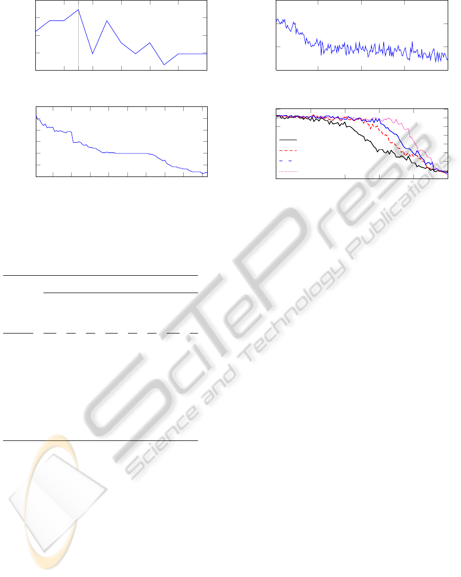
In Fig. 5(a) one can observe that the recognition

rate during classiﬁcation had a maximum peak at

= 3

, which argues for a high degree of discrim-

inability. This is emphasized by the vertical line in

Fig. 5(a). Without using any eigenvectors, only the

mean shape is taken into account during feature ex-

traction, which leads to lower discriminability. Using

more eigenvectors would cause a more exact recon-

struction of the skeleton conﬁguration and therefore a

smaller discriminability due to the increased coverage

of variability.

For simplicity, we used the

Nearest Neighbor

(

-NN) framework for classiﬁcation, which assigns a

class label to a feature vector employing an arbitrary

SCALE-INDEPENDENT SPATIO-TEMPORAL STATISTICAL SHAPE REPRESENTATIONS FOR 3D HUMAN

ACTION RECOGNITION

291

0 2 4

8 10 12

0.89

0.9

0.91

0.92

0.93

(a) Number of eigenvectors k

Overall recognition rate

10 20 30 40

50 60

70 80 90

0.4

0.5

0.6

0.7

0.8

0.9

(b) Number of neighbors k

Overall recognition rate

Figure 5: Effect of increasing (a) the number of eigenvectors

used for building the feature vector and (b) the number of

neighbors for k-NN classiﬁcation on recognition rates.

Table 4: Confusion matrix with overall recognition rates

obtained by exhausting leave-one-out test on our dataset.

Training Testing

walking

running

marching

sneaking

hopping

jumping

golfing

salsa

walking 100 0 0 0 0 0 0 0

running 33 56 0 11 0 0 0 0

marching 4 0 93 0 0 4 0 0

sneaking 0 0 0 100 0 0 0 0

hopping 13 7 0 0 80 0 0 0

jumping 0 0 7 7 0 86 0 0

golfing 0 0 0 0 0 0 100 0

salsa 0 0 3 0 0 0 0 97

distance measure

d(y

test

, y

target

)

between the feature

vector

test

and a representative prototype vector

target

In our experiments, we chose the Euclidean distance

d(y

test

, y

target

) = ky

test

− y

target

As can be seen in Fig. 5(b), using

k = 1

gave the

best recognition rate, while increasing the number of

neighbors caused apparent worse results as well as

higher computational time for classiﬁcation.

Using this feature extraction scheme and the

-NN

classiﬁer, we were able to achieve results as shown

in the confusion matrix obtained by exhaustive leave-

one-out test in Tab. 4. As one can see, most of the

action classes in our dataset were recognized correctly

in more than

80%

of the cases, while

classes gave

recognition rates of nearly

100%

. Solely the action

class

running

has been confused with the semanti-

0.88

0.9

0.92

0.94

(a) Gaussian noise variance σ

gauss

Overall recognition rate

0 0.2 0.4

0.6

0.8 1

0.2

0.3

0.4

0.5

0.6

0.7

0.8

0.9

(b) Amount of Salt-and-Pepper noise p

Overall recognition rate

not ﬁltered

median

= 3

median

= 5

median

= 15

Figure 6: Inﬂuence of increasing the strength of (a) zero-

mean gaussian noise and (b) Salt-and-Pepper noise to the

recognition rates. In order to reduce this performance drop

in (b), a temporal median ﬁlter of size

median

was applied

on the data as a preprocessing step.

cally related classes

walking

and

sneaking

due to

their similar variations during execution.

3.4 Robustness to Noise

In real-world applications the input data for action

classiﬁcation are not ideal. Hence we modeled the

inﬂuence of additive, zero-mean normally distributed,

and uncorrelated Salt-and-Pepper noise to quantita-

tively evaluate the robustness of our approach.

As can be seen in Fig. 6(a), adding Gaussian noise

to the input data did not negatively affect the classiﬁ-

cation results. This might be explained by the mean

subtraction on the one hand and the usage of PCA on

the other hand during modeling. In order to ﬁnd the

principal components, noise added to the data will only

affect the eigenvectors corresponding to the smaller

eigenvalues, while the inherent and consistent infor-

mation of movement over time is still captured by the

eigenvectors corresponding to the larger eigenvalues.

A similar behavior can be observed in the case

of adding uncorrelated Salt-and-Pepper noise to input

data. As can be seen in Fig. 6(b), while the recogni-

tion rates were decreasing with the amount of added

noise, simple median ﬁlters applied to the single chan-

nels along the time dimension were able to drastically

reduce these effects. It can be seen that an amount

70%

Salt-and-Pepper noise can be handled by ap-

plying a

-frame temporal median ﬁlter which only

results in a small decrease in the recognition rates.

ICPRAM 2012 - International Conference on Pattern Recognition Applications and Methods

292

Table 5: Effects of integrating temporal context into our

model. Since the model became more distinctive regarding

the execution speed of actions, integrating these temporal

information affected the recognition rates slightly.

Historical Offset ∆

hist

Number of History Frames k

hist

1 2 3 4

5 92.45 92.45 91.82 91.19

10 93.08 92.45 91.82 92.45

15 91.82 91.19 91.82 91.82

30 90.57 89.31 92.45 89.94

3.5 Comparison to Other Work

Although human action recognition was widely in-

vestigated for 2d data, there is less work available

concerning the case of having access to 3d data. A

similar approach to classify human actions in 3d data

was taken in (Han et al., 2010), but they selected less

action classes from the CMU MoCap dataset. While

they distinguish only 3 action classes with small varia-

tions in execution, recognition rates of

98.29%

were

obtained without taking the presence of noise into ac-

count. In (Junejo et al., 2011), the same database has

been used to create artiﬁcial 2d views and evaluating

several distance metrics on the landmark points with-

out modeling the shape at all. They observed recogni-

tion rates of about

90.5%

in average when combining

all their camera views for training and testing. The

approach of (Shen et al., 2008) employed homography

constraints and lead to an overall recognition rate of

about 92% .

Compared to those results, our approach performs

similarly (

92.45%

) on the same data even in the pres-

ence of noise.

3.6 Use of Temporal Context

As mentioned in Sec. 2.2, we not only model the varia-

tions of landmark transitions during a ﬁxed time period,

but also integrate the evolution of these movements by

incorporating the temporal context during an action

execution.

Tab. 5 shows that the integration of temporal infor-

mation into the action model affects the recognition

rates slightly. We tested several values for the number

of history frames

hist

integrated to the model as well

as the temporal offset

∆

hist

= (t

−t

i−1

), 1 ≤ i ≤ t

hist

these frames. The observed behavior can be explained

by taking into account the variability of action execu-

tions within the dataset, where, for example, one actor

performs slower while another performs faster.

Although this fact is not requested in the given

scenario, it would allow us to distinguish actions re-

garding the execution speed which can be of inter-

est in further applications. For instance, the confu-

sion between action classes

running

and

walking

sneaking

could be dissolved exploiting these tempo-

ral information.

4 SUMMARY AND OUTLOOK

We proposed a method for representing sequences of

human actions while integrating spatial and temporal

information into a combined model. This representa-

tion scheme was shown to be suitable for human action

classiﬁcation applications. Experiments performed on

the CMU motion capturing dataset gave promising re-

sults which are able to compete with existing state of

the art approaches.

To overcome certain false classiﬁcations, a hierar-

chy of single binary classiﬁers can be built. One can

observe that similar motions are grouped into closer

subtrees, while diverging actions are located in distinct

subtrees.

Another ﬁeld of research is the design of fea-

tures used for classiﬁcation. Since closely related

classes tend to be confused, more sophisticated fea-

tures should help to overcome this behavior.

The parameter vector

could be used to build

a self-similarity matrix instead of using the Euclid-

ian landmark distances as proposed by (Junejo et al.,

2011). More sophisticated distance measures like the

angular distance in the manifold space could beneﬁt

the discriminability of the action classes.

For feeding real-world data to our approach, skele-

ton conﬁgurations can be extracted from frames pro-

vided by depth measuring camera devices such as Mi-

crosoft Kinect or PMD, which was recently shown to

be possible in real-time (Li et al., 2010; Shotton et al.,

2011). The combination of Active Shape Model based

landmark detection and our proposed action represen-

tation could also be promising.

ACKNOWLEDGEMENTS

The data used in our experiments was obtained from

mocap.cs.cmu.edu

. The database was created with

funding from NSF EIA-0196217.

REFERENCES

Bookstein, F. L. (1997). Landmark methods for forms with-

out landmarks: Morphometrics of group differences in

SCALE-INDEPENDENT SPATIO-TEMPORAL STATISTICAL SHAPE REPRESENTATIONS FOR 3D HUMAN

ACTION RECOGNITION

293

outline shape. Medical Image Analysis, 1(3):225–243.

Bosch, J., Mitchell, S., Lelieveldt, B., Nijland, F., Kamp,

O., Sonka, M., and Reiber, J. (2002). Automatic seg-

mentation of echocardiographic sequences by active

appearance motion models. IEEE Transactions on

Medical Imaging, 21(11):1374–1383.

Cootes, T. F., Taylor, C. J., Cooper, D. H., and Graham, J.

(1995). Active shape models—their training and ap-

plication. Computer Vision and Image Understanding,

61:38–59.

Dollar, P., Rabaud, V., Cottrell, G., and Belongie, S. (2005).

Behavior recognition via sparse spatio-temporal fea-

tures. In Proceedings of the 2

Joint IEEE Interna-

tional Workshop on Visual Surveillance and Perfor-

mance Evaluation of Tracking and Surveillance, pages

65–72. IEEE Computer Society.

Gavrila, D. (1999). The visual analysis of human movement:

A survey. Computer Vision and Image Understanding,

73(1):82–98.

Gorelick, L., Blank, M., Shechtman, E., Irani, M., and Basri,

R. (2007). Actions as space-time shapes. IEEE Trans-

actions on Pattern Analysis and Machine Intelligence,

29(12):2247–2253.

Haase, D. and Denzler, J. (2011). Anatomical landmark

tracking for the analysis of animal locomotion in x-ray

videos using active appearance models. In Heyden, A.

and Kahl, F., editors, Image Analysis, volume 6688 of

Lecture Notes in Computer Science, pages 604–615.

Springer Berlin / Heidelberg.

Han, L., Wu, X., Liang, W., Hou, G., and Jia, Y. (2010).

Discriminative human action recognition in the learned

hierarchical manifold space. Image and Vision Com-

puting, 28(5):836–849.

Jia, K. and Yeung, D.-Y. (2008). Human action recognition

using local spatio-temporal discriminant embedding.

In Proceedings of the IEEE Conference on Computer

Vision and Pattern Recognition, pages 1–8.

Junejo, I., Dexter, E., Laptev, I., and Perez, P. (2011). View-

independent action recognition from temporal self-

similarities. IEEE Transactions on Pattern Analysis

and Machine Intelligence, 33(1):172–185.

Ke, Y., Sukthankar, R., and Hebert, M. (2007). Spatio-

temporal shape and ﬂow correlation for action recogni-

tion. In Proceeding of the IEEE Conference on Com-

puter Vision and Pattern Recognition, Visual Surveil-

lance Workshop, pages 1–8.

Laptev, I. (2005). On space-time interest points. Interna-

tional Journal of Computer Vision, 64(2-3):107–123.

Lelieveldt, B. P. F.,

umc

u, M., van der Geest, R. J., Reiber,

J. H. C., and Sonka, M. (2003). Multi-view active

appearance models for consistent segmentation of mul-

tiple standard views: application to long and short-axis

cardiac mr images. In Proceedings of the 17

Interna-

tional Congress and Exhibition on Computer Assisted

Radiology and Surgery, pages 1141–1146.

Li, W., Zhang, Z., and Liu, Z. (2010). Action recognition

based on a bag of 3d points. In Proceedings of the IEEE

Computer Society Conference on Computer Vision and

Pattern Recognition Workshops, pages 9–14.

Oost, E., Koning, G., Sonka, M., Oemrawsingh, P., Reiber, J.,

and Lelieveldt, B. (2006). Automated contour detection

in x-ray left ventricular angiograms using multiview

active appearance models and dynamic programming.

IEEE Transactions on Medical Imaging, 25(9):1158–

1171.

Poppe, R. (2010). A survey on vision-based human action

recognition. Image and Vision Computing, 28(6):976–

990.

Schwarz, L. A., Mateus, D., Castaneda, V., and Navab, N.

(2010). Manifold learning for tof-based human body

tracking and activity recognition. In Proceedings of the

British Machine Vision Conference, pages 80.1–80.11.

BMVA Press.

Schwarz, L. A., Mateus, D., and Navab, N. (2012). Recog-

nizing multiple human activities and tracking full-body

pose in unconstrained environments. Pattern Recogni-

tion, 45(1):11–23.

Shen, Y., Ashraf, N., and Foroosh, H. (2008). Action recogni-

tion based on homography constraints. In Proceedings

of the 19

International Conference on Pattern Recog-

nition, pages 1–4.

Shotton, J., Fitzgibbon, A. W., Cook, M., Sharp, T., Finoc-

chio, M., Moore, R., Kipman, A., and Blake, A. (2011).

Real-time human pose recognition in parts from single

depth images. In Proceddings of the IEEE Conference

on Computer Vision and Pattern Recognition, pages

1297–1304.

Sun, M.-F., Wang, S.-J., Liu, X.-H., Jia, C.-C., and Zhou,

C.-G. (2011). Human action recognition using tensor

principal component analysis. In Proceedings of the 4

IEEE International Conference on Computer Science

and Information Technology, pages 487–491.

Turaga, P., Chellappa, R., Subrahmanian, V., and Udrea, O.

(2008). Machine recognition of human activities: A

survey. IEEE Transactions on Circuits and Systems for

Video Technology, 18(11):1473–1488.

Wang, L. and Suter, D. (2007). Learning and matching of

dynamic shape manifolds for human action recognition.

IEEE Transactions on Image Processing, 16(6):1646–

1661.

Yamazaki, M., Chen, Y.-W., and Xu, G. (2007). Human

action recognition using independent component anal-

ysis. In Intelligence Techniques in Computer Games

and Simulations.

Zhang, J., Li, S. Z., and Wang, J. (2005). Manifold learn-

ing and applications in recognition. In Tan, Y.-P.,

Yap, K., and Wang, L., editors, Intelligent Multime-

dia Processing with Soft Computing, volume 168 of

Studies in Fuzziness and Soft Computing, pages 281–

300. Springer-Verlag.

ICPRAM 2012 - International Conference on Pattern Recognition Applications and Methods

294