BRKGA ADAPTED TO MULTIOBJECTIVE UNIT COMMITMENT

Solving Pareto Frontier for UC Multiobjective Problem using BRKGA SPEA2

NPGA and NSGA II Techniques

Lu´ıs A. C. Roque

, Dalila B. M. M. Fontes

and Fernando A. C. C. Fontes

ISEP-DEMA/GECAD, Instituto Superior de Engenharia do Porto, Porto, Portugal

FEP/LIAAD-INESC Porto L.A., Universidade do Porto, Porto, Portugal

FEUP/ISR-Porto, Universidade do Porto, Porto, Portugal

Keywords:

Unit comitment, Genetic algorithm, Multi objective optimization, Pareto optimal curves.

Abstract:

The environmental concerns are having a signiﬁcant impact on the operation of power systems. The traditional

Unit Commitment problem, which to minimizes the fuel cost is inadequate when environmental emissions

are also considered in the operation of power plants. This paper presents a Biased Random Key Genetic

Algorithm (BRKGA) approach combined with non-dominated sorting procedure to ﬁnd solutions for the unit

commitment multiobjective optimization problem. In the ﬁrst stage, the BRKGA solutions are encoded by

using random keys, which are represented as vectors of real numbers in the interval [0, 1]. In the subsequent

stage, a non-dominated sorting procedure similar to NSGA II is employed to approximate the set of Pareto

solution through an evolutionary optimization process. The GA proposed is a variant of the random key genetic

algorithm, since bias is introduced in the parent selection procedure, as well as, in the crossover strategy. Test

results with the existent benchmark systems of 10 units and 24 hours scheduling horizon are presented. The

comparison of the obtained results with those of other Unit Commitment (UC) multiobjective optimization

methods reveal the effectiveness of the proposed method.

1 INTRODUCTION

The power system generation scheduling is composed

of two tasks: On the one hand, the traditional unit

commitment (UC) that involves scheduling the turn-

on and turn-off of the thermal generating units; on the

other hand, the economic dispatch (ED), which as-

signs, the amount of power that should be produced

by each on-line unit in order to minimize the total

operating costs for a speciﬁc time generation hori-

zon. The traditional conﬁguration of this problem was

modiﬁed when environmental concerns arised due to

the goals imposed by Kyoto protocol. The carbon

emissions produced by fossil-fueled thermal power

plants should also be minimized. Hence, it is nec-

essary to consider the emission as another objective.

Therefore, we are in the presence of problem with

two, usually conﬂicting, objectives.

Several methods have been reported in the liter-

ature concerning to the environmental/economic dis-

patch problem. However, to obtain an optimal solu-

tion, it is important to consider not only the output

generation level of each generating unit but also the

turn on/off schedule, due to start-up costs/emissions

that havesigniﬁcant inﬂuence in the problem solution.

In (Granelli et al., 1992) the problem is formulated

as single objective with an emission limit constraint.

The disadvantage of such an approach is that it does

not allow for obtaining solutions with a tradeoff be-

tween costs and emissions. In addition, this type of

approach leads to solutions maximizing the proﬁt but

disregarding possible solutions with CO2 reduction.

The ε-constraint method for multiobjective opti-

mization was presented in (Hsiao et al., 1994). This

method is based on preferences of the objectives. The

most important objectives are considered while the

other objectives are treated as constraints bounded by

some allowable levels. The main disadvantage of this

approach is to ﬁnd weakly non-dominated solutions.

Some of the previous studies of unit commit-

ment problems including emission constraints have

been solved using lagrange relaxation methods (Wang

et al., 1995; Yamin et al., 2007). In (Wang et al.,

1995) an augmented lagrange relaxation is used

to solve a unit commitment considering the typi-

cal system constraints such as power balance, min-

A. C. Roque L., B. M. M. Fontes D. and A. C. C. Fontes F..

BRKGA ADAPTED TO MULTIOBJECTIVE UNIT COMMITMENT - Solving Pareto Frontier for UC Multiobjective Problem using BRKGA SPEA2 NPGA

and NSGA II Techniques.

DOI: 10.5220/0003759500640072

In Proceedings of the 1st International Conference on Operations Research and Enterprise Systems (ICORES-2012), pages 64-72

ISBN: 978-989-8425-97-3

 2012 SCITEPRESS (Science and Technology Publications, Lda.)

imum up/down time and ramp rate constraints and

adding transmission and environmental constrains. In

(Yamin et al., 2007) lagrange relaxation is combined

with evolutionary programming.

Current research is directed to handle both ob-

jectives simultaneously as competing objectives in-

stead of simplifying the multiobjective problem to a

single objective problem. Three multiobjective evo-

lutionary algorithms (MOEAs) have been applied to

the Economic Dispatch (ED) problem with meaning-

ful success (Abido, 2003c; Abido, 2003b; Abido,

2003a). Since they use a population of solutions

in their search, multiple Pareto-optimal solutions

can, in principle, be found in one single run. Dif-

ferent MOEAs like Niched Pareto Genetic Algo-

rithm (NPGA) (Horn et al., 1994), Strength Pareto

Evolutionary Algorithm (SPEA) (Zitzler and Thiele,

1998) and Non-dominated Sorting Genetic Algorithm

(NSGA) (Srinivas and Deb, 1994) have been applied

to this problem. These models can be efﬁciently

used to eliminate most of the difﬁculties of classical

methods. However, the quality and diversity of the

nondominated solutions presented in (Abido, 2003c;

Abido, 2003b; Abido, 2003a) have not been measured

and assessed quantitively. In (Abido, 2006) a com-

parative study among MOEA techniques was devel-

oped to evaluate their potential to solve the multiob-

jective ED problem. The potential of MOEA to han-

dle this problem is investigated and their effectiveness

to solve the ED multiobjective problem was shown.

It is important to refer that new versions of MOEAs

were presented such as NSGA-II (Deb et al., 2002),

and SPEA2 (Zitzler et al., 2001). The NSGA-II algo-

rithm was also applied to the ED multiobjective prob-

lem in (Basu, 2008).

Gonc¸alves and Resende (2010) introduce the tuto-

rial on the implementation and use of Biased Random

Key Genetic Algorithm (BRKGA) for solving com-

binatorial optimization methods. More recently, in

(Roque et al., 2011) the BRKGA approach is used to

ﬁnd solutions for single objective Unit Commitment

problem.

In this paper the BRKGA algorithm combined

with nondominated sorted procedure and MOEA

techniques is applied to the two standard 10-unit 24-

hour test systems presented in (Winter et al., 2003)

and (Sawaragi et al., 1985). The proposed ap-

proach BRKGA is combined with a ranking selection

method, that is used to focus on different levels of the

nondominated solutions, and a sharing ﬁtness proce-

dure as in NSGA.

The paper is organized as follows: Following

the description of the problem formulation, which is

given in section 2, an explanation on the BRKGA and

its implementation to the UC bi-objective problem, is

given in section 3. Section 4 provides test results and

ﬁnally in Section 5 some conclusions are drawn.

2 UC MULTIOBJECTIVE

PROBLEM FORMULATION

In the multiobjective UC problem one needs to de-

termine an optimal schedule, which minimizes the

production cost and emission of atmospheric pollu-

tants over the scheduled time horizon subject to sys-

tem and operational constraints. Due to its combina-

torial nature, multi-period characteristics, and nonlin-

earities, the UC problem is a hard optimization prob-

lem, which involves both integer and continuous vari-

ables and a large set of constraints.

Let us now introduce the parameters and variables

notation.

Decision Variables:

t,j

: Thermal generation of unit j at time period t, in [MW];

t,j

: Status of unit j at time period t (1 if the unit is on; 0

otherwise);

Auxiliary Variables:

on/off

(t): Time periods for which unit j has been continu-

ously on-line/off-line until time period t, in [hours];

Parameters:

T: Number of time periods (hours) of the scheduling time

horizon;

t: Time period index;

N: Number of generation units;

j: Generation unit index;

: System spinning reserve requirements at time period t,

in [MW];

: Load demand at time period t, in [MW];

Ymin

: Minimum generation limit of unit j, in [MW];

Ymax

: Maximum generation limit of unit j, in [MW];

: Number of the base units;

on/off

min,j

: Minimum uptime/downtime of unit j, in [hours];

c,j

: Cold start time of unit j, in [hours];

H/C,j

: Hot/Cold start-up cost of unit j, in [$];

: Shut down cost of unit j, in [$];

e,j

: Start-up atmospheric pollutant emission of unit j, in

[ton−CO2] if CO2 or [mg/Nm

] if nitrogen oxides;

∆

dn/up

: Maximum allowed output level decrease/increase

in consecutive periods for unit j, in [MW];

2.1 Objective Functions

As already said, in the multi-objective problem for-

mulation, two important objectives in electrical ther-

mal power system are considered. These are economy

and environmental impacts.

On the one hand, the ﬁrst objective is to minimize

the system operation costs composed by generation

and start-up costs. The generation costs, i.e. the fuel

costs, are conventionally given by a quadratic cost

function as in equation (1),

BRKGA ADAPTED TO MULTIOBJECTIVE UNIT COMMITMENT - Solving Pareto Frontier for UC Multiobjective

Problem using BRKGA SPEA2 NPGA and NSGA II Techniques

t, j

) = a

· (Y

t, j

)

+ b

·Y

t, j

+ c

, (1)

where a

are the cost coefﬁcients of unit j.

Therefore, the cost incurred with an optimal

scheduling is given by the minimization of the total

costs for the whole planning period, as in equation

(2).

Minimize

∑

t=1

∑

j=1

(Yth

t, j

) · u

t, j

(2)

+ SU

t, j

· (1− u

t−1, j

) · u

t, j

(3)

+SD

· (1− u

t, j

) · u

t−1, j

}

where S

t, j

and SD

t, j

are the start-up and shut-down

costs of unit j at time period t, respectively.

On the other hand, the second objective is to

minimize the total quantity of atmospheric pollutants

emission. The emissions are generally expressed as a

quadratic function:

t, j

) = α

· (Y

t, j

)

+ β

·Y

t, j

+ γ

, (4)

where α

,β

,γ

are the emission coefﬁcients of unit j.

So, the total emission of atmospheric pollutants is

expressed as follows:

Minimize

∑

t=1

∑

j=1

(Yth

t, j

) · u

t, j

(5)

+Se

t, j

· (1− u

t−1, j

) · u

t, j

}

where Se

is the start-up atmospheric pollutant emis-

sions of unit j at time period t.

2.2 Constraints

The constraints can be divided into two sets: the de-

mand constraints and the technical constraints. Re-

garding the ﬁrst set of constraints it can be further

divided into load requirements and spinning reserve

requirements, which can be written as follows:

1) Power Balance Constraints.

The total power generated must cover the total load

demand, for each time period.

∑

j=1

t, j

· u

t, j

≥ D

,t ∈ {1,2,...,T}. (6)

2) Spinning Reserve Constraints.

The spinning reserve is the total amount of real power

generation available from on-line units net of their

current production level.

∑

j=1

Ymax

· u

t, j

≥ R

+ D

,t ∈ {1, 2, ...,T}. (7)

The second set of constrains includes unit output

range, minimum number of time periods that the unit

must be in each status (on-line and off-line), and the

maximum output variation allowed for each unit.

3) Unit Output Range Constraints.

For each time period t and unit j, the real power out-

put of each generator is restricted by maximum and

minimum production limits.

Ymin

· u

t, j

≤ Y

t, j

≤ Ymax

· u

t, j

. (8)

4) Ramp Rate Constraints.

Due to the thermal stress limitations and mechanical

characteristics, the output variation levels of each on-

line unit in two consecutive periods are restricted by

ramp rate limits.

−∆

≤ Y

t, j

−Y

t−1, j

≤ ∆

. (9)

5) Minimum Uptime/Downtime Constraints.

If the unit has already turned on or off, there will be

a minimum uptime/downtime time before it is shut-

down or started-up, respectively.

(t) ≥ T

min, j

and T

of f

(t) ≥ T

of f

min, j

. (10)

3 MULTIOBJECTIVE UC

OPTIMIZATION

3.1 Decoding Procedure

The decoding procedure is commonly used in all

four multiobjective optimization algorithms. For

each chromosome, the corresponding solution is per-

formed in two main stages, as it can be seen in Figure

2 in (Roque et al., 2011). Firstly, the output genera-

tion level matrix for each unit and period is computed

from random key value. In this solution, the units

production is proportional to their priority, which is

given by the random key value. By doing so, each

element of the output generation matrix, Y

t, j

is given

as the product of the percentage vectors by the peri-

ods demand D

. Here each component of the percent-

age vectors are given by corresponding random key

entrie divided by the sum of the all random key val-

ues as illustrated in algorithm 1 (Roque et al., 2011).

Then, these solutions are checked for constraints sat-

isfaction using a repair algorithm presented in (Roque

et al., 2011).

ICORES 2012 - 1st International Conference on Operations Research and Enterprise Systems

3.2 Repair Algorithm

The idea of this technique is to convert any infeasi-

ble individuals to a feasible solution by repairing the

sequential possible violations constraints in the UC

problem. The repair algorithm is composed by several

steps. Firstly, the output levels are adjusted in order

to satisfy the output range constraints. Next, we have

the adjustment of output levels to satisfy ramp rate

limits. It follows the repairing of the minimum up-

time/downtime constraints violation. Afterwards, the

output levels are adjusted in order to satisfy spinning

reserve requirements. Finally, the output levels are

adjusted for demand requirements satisfaction at each

time period. For details about the repairing mecha-

nisms, the reader is refered to (Roque et al., 2011).

3.3 NSGA

A fast and elitist non-dominated sorted genetic algo-

rithm (NSGA II) (Deb et al., 2002) is used to approx-

imate the set of Pareto solution. In this approach,

the ranking selection method is used to focus on non-

dominated solutions while the crowding distance is

computed to ensure diversity along the nondominated

front. The population of size N

is used for selec-

tion, crossover,and mutation to create a new offspring

population of equal size. The rank procedure is em-

ployed by different levels of domination until all in-

dividuals in the intermediate combined population, of

size 2N

, are ranked. Firstly, the nondominated solu-

tions are assigned with same rank value and thereafter

the crowding distance is computed. The nondomi-

nated solutions must be emphasized more than any

other solution. In order to ﬁnd individuals of the next

front, the solutions of the ﬁrst front are temporarily

ignored, and the above procedure is repeated to ﬁnd

subsequent fronts. The individuals of the new popu-

lation are selected from the intermediate population,

they are chosen from subsequent nondominatedfronts

in the order of their ranking. To choose exactly the

population members, the solutions of the last front are

sorted considering the crowding distance by descend-

ing order. The NSGA-II approach proposed by (Deb

et al., 2002) was implementated as follows:

• Generate random population, decoding the indi-

viduals and evaluate the solutions;

• Sort the population using non-domination-sort.

For each individual, rank and crowding distance

are assigned;

• For each generation the follows steps are given:

Select the parents, which are ﬁt for reproduction

by using the binary tournament selection based on

the rank and crowding distance; genetic operators

copy, simulated binary crossover and mutation are

applied under selected parents; the offspring pop-

ulation is combined with parents (the size of in-

termediate population is the double); selection is

performed to set the individuals of the next gen-

eration; after sorting the intermediate population

, only the best individuals are selected based on

its rank and crowding distance; a new generation

is then obtained mantaining the population size

ﬁxed; the algorithm stop criterium is the max-

imum number of generations previously estab-

lished.

3.4 NPGA

A Niched pareto genetic algorithm was presented in

(Horn et al., 1994). This thecnique involves the addi-

tion of two specialized genetic operators: Pareto dom-

ination tournaments and ﬁtness sharing. These oper-

ators allow for selection based on partial ordering of

the population, as well as, to preserve diversity in the

population.

Tournament selection is used to adjust selection

pressure by changing the tournament size. Two can-

didates are chosen at random from the current popu-

lation. A comparison set of tdom individuals is also

chosen randomly. Each of the candidates are com-

pared to each individual in the comparison set. If a

candidate is dominated by the comparison set, and

other is not, it loses the competition. If there are tour-

nament ties, i.e. neither or both are dominated by the

comparison set, the decision is based on the ﬁtness

sharing of individuals, using niche counts as calcu-

lated for the objective space in (Horn et al., 1994).

Each canditate niche count is computed in the objec-

tive space, using its evaluated objective values. The

candidate with lowest niche count wins the tourna-

ment. Tournaments are held until the next generation

is ﬁlled. Then crossover and mutation operators are

applied to the new population. As already said, in the

case of a tie, the population density around each can-

didate is computed within a speciﬁed distance, known

as the niche radius σ

. The niche count for candi-

date i is given by:

(

∑

j∈Pop



1−

i, j



i, j

< σ

i, j

>= σ

(11)

The winner of the tied tournament is the competi-

tor with the lowest niche count. As in (Horn et al.,

1994), the ﬁtness sharing is updated continuously,

once the niche counts are calculated using individuals

in the partially ﬁlled population of the next genera-

BRKGA ADAPTED TO MULTIOBJECTIVE UNIT COMMITMENT - Solving Pareto Frontier for UC Multiobjective

Problem using BRKGA SPEA2 NPGA and NSGA II Techniques

tion, rather than that of the current generation.

3.5 SPEA

The Strenght Pareto Evolutionary Algorithms

(SPEAs) was introduced in (Zitzler and Thiele,

1998) and an improve version, known as SPEA II

is given in (Zitzler et al., 2001). In this algorithm,

nondominated solutions are stored in an external

set. The individuals are assigned according to the

Pareto dominance concept. When the nondominated

solutions exceds a previously ﬁxed size for the

external set, the number of individuals in the external

set is reduced by means of a truncation thecnique, as

in (Zitzler et al., 2001). If the number of nondomi-

nated individuals is less than the predeﬁned external

set size, the external set is ﬁlled up by dominated

individuals. The ﬁtness assignment occurs in two

different stages. The individuals are assigned by the

strengths of its dominators in both the external set

and the population. Strenght represents the number

of individuals in the population and in the external set

covered by individual considered. The ﬁtness of each

individual is given by the sum of the strenghts of its

dominators in the external set and in the population.

If individuals have equal ﬁtness value, the density

estimation technique, as given in SPEA2 (Zitzler

et al., 2001), is used. This technique results from an

adaptation of the k−th nearest neighbor method. The

basic idea of the truncation procedure is to remove

the individual which has the minimum distance to

another individual. If there are several individuals

with minimum distance, the individuals with second

smallest distances to another individual are removed

and so on. The SPEA-II approach proposed by

(Zitzler et al., 2001) implementates the following

steps:

• Generate the initial population, decoding the indi-

viduals and evaluate the solutions and create the

empty external pareto-optimal;

• Compute ﬁtness values of individuals in the pop-

ulation and in the external set;

• Copy nondominated individuals of the population

to the external set;

• For each generation: Update the external set keep-

ing only the nondominated solutions. When the

number of nondominated solutions is higher than

the speciﬁed size for the external set, it is reduced

by applying the truncation thecnique. If the num-

ber of nondominated individuals is less than the

external set size, the external set is ﬁlled up by

dominated individuals;

• The mating pool is ﬁlled using binary tournament

selection with replacement on the updated exter-

nal set;

• After the recombination, of the mating pool, the

crossover and mutation operators are applied and

a new population is created;

• The algorithm stops when the maximum number

of generations is reached.

3.6 BRKGA adapted to Multiobjective

UC Optimization

We also use the ranking selection method for ordering

the nondominated solutions according to the Pareto

domination concept while the crowding distance is

used to break ties by chosing the best indiduals to

be included in new population. For details about the

BRKGA approach, the reader is refered to (Gonc¸alves

and Resende, 2010; Roque et al., 2011). The ini-

tial population with size N

is criated by generating

the random keys. Given population of chromosomes

(random keys) a decoding procedure is applied such

that at each chromosome corresponds a feasible UC

solution, that is an output generation level matrix and

the corresponding unit status matrix both satisfying

the UC constraints. The ﬁtness function used to eval-

uate the solutions includes both the total operational

costs and CO2 emissions. We adopt a ﬁtness proce-

dure similar to that of NSGA-II, given in (Deb et al.,

2002). Therefore, the population is sorted based on

the nondomination. Each solution is assigned a ﬁt-

ness (rank) equal to its nondomination level. The bi-

ased selection and biased crossover operators and the

introduction of mutants are used to create a offspring

population, also of size N

. On the one hand, the bi-

ased selection ensures that one of the parents used for

mating comes from a subset containing the best so-

lutions of the current population. On the other hand,

the biased crossover chooses with higher probability

an allele from the best parent. Mutants are generated

as the initially population and are introduced directely

on the next generation.

We start by combining the current population with

the newly obtained one. The combined population

size is the double (2N

) of the current population and

it is sorted by the nondomination criterium (Fast Non-

dominated Sorting Approach).

The nondomination criterium leads to several lev-

els of nondominated fronts. For the ﬁrst level, the

nondominated individuals of the combined popula-

tion are chosen. Second level, corresponds to a front

containing individuals only dominated by the individ-

uals of the ﬁrst level front. All other levels are deﬁned

ICORES 2012 - 1st International Conference on Operations Research and Enterprise Systems

in a similar way, that is, in each level a front contain-

ing individuals dominated by all previous nondomi-

nated fronts is obtained. In order to obtain the new

population we go through the generated fronts, in as-

cending order of level, and include all its individuals

until we reach N

. At the last nondominated front

level to be included if only some of the individuals

are to be chosen, the descending order of crowding

distance is used as a selection criterium.

The multiobjective BRKGA ﬂowchart is illus-

trated in Figure 1.

Entry

Generation of

random key vectors

All

generations?

Exit

Generate mutants

Biased crossover

Classify

as elit or non-elite

Crowding distance

assignment

Fast Nondominated

Sorting Approach

Combine new population

and current population

Sort new

population

Evaluate

Select Parents

Copy elit

Decoding:

Generate a feasible solution

New

population

Figure 1: Flowchart of BRKGA multiojective algorithm.

3.6.1 Genetic Operators in BRKGA

Biased Selection: Pair of parents are selected from

parent population. The parent population is divided

into two sets: The elit set, comprising the best indi-

viduals, and the non-elit set, comprising the remain-

ing individuals. One parent is selected from the elit

set, while the other parent is chosen from the remain-

ing, non-elite, individuals.

Biased Crossover. Given two parents and a spec-

iﬁed probability of crossover, the crossover inter-

changes the genes or alleles to produce a new individ-

ual. As already mentioned, genes are chosen by using

a biased uniform crossover, that is, for each gene a

biased coin is tossed to decide on which parent the

gene is taken from. This way, the offspring inherits

the genes from the elite parent with higher probabil-

ity (0.7 in our case).

Mutants. To ensure diversity and to avoid prema-

ture convergence, we introduce a percentage of new

individuals, called mutants, in the population. These

individuals are randomly generated as was the case

for the initial population.

4 COMPUTATIONAL

EXPERIMENTS AND RESULTS

4.1 GA Parameters

4.1.1 BRKGA Conﬁguration

The BRKGA ﬁnal parameter values were decided

after some empirical experiments have been per-

formed. The experimented values were chosen using

the guidelines provided by (Gonc¸alves and Resende,

2010; Deb et al., 2002), as well as, the computational

experiments in (Roque et al., 2011). The current pop-

ulation of solutions is evolved by the GA operators

onto a new population as follows:

Elit set is formed by 20% of best solutions; 40%

of the new population is obtained by introducing mu-

tants; Finally, the remaining 60% of the population

is obtained by biased reproduction, which is accom-

plished by having both a biased selection and a biased

crossover. Moreover, we set the number of genera-

tions to 100 (10N), the population size to 40(4N) and

the crossover probability to 0.7.

4.1.2 SPEA, NSGA, and NPGA Conﬁgurations

The algorithms are implemented according to their

description in the literature. The other operators (re-

combination, mutation, sampling) remain identical.

To ensure the same conditions of application of the

method BRKGA, identical population size of 40 and

number of generations of 100 to BRKGA are used for

each algorithm.

The NPGA, NSGA II, and SPEA2 parameters val-

ues are choosen using the guidelinesproposed in (Deb

et al., 2002). Some complementary computational ex-

periments are performed, where other appropriate val-

ues of the GA parameters are arrived at based on the

satisfactory performance of trials conducted for this

application with different range of values. For NPGA,

the niche radius σ

= 0.1 was choosed as in (Horn

et al., 1994) and several computational experiments

were made in order to choose the size of the compar-

ison set t

dom

. The parameter ranges between 5% and

30%. The results obtained have shown a favorable

value of t

dom

to be 10%.

For NPGA and NSGA II real coding an intermedi-

ate crossover similar to Matlab crossover operator has

been employed. The childs are obtained as Child

Parent

+ rand.ratio.(Parent

− Parent

) and

BRKGA ADAPTED TO MULTIOBJECTIVE UNIT COMMITMENT - Solving Pareto Frontier for UC Multiobjective

Problem using BRKGA SPEA2 NPGA and NSGA II Techniques

Child

= Parent

− rand.ratio.(Parent

− Parent

)

where rand is random number in the interval [0,1], the

ratio crossover was set 1.2 and the crossover probabil-

ity to 0.8. The Gaussian mutation is used as in Matlab

Toolbox Opimization with scale = 0.1,shrink = 0.5.

The mutation rates has been set to 0.2.

For SPEA2, we use a population of size 40 and an

external population of size 40, so that overall popu-

lation size becomes 80. The uniform crossover and

simulated binary crossover operators are applied with

probability 0.7 and 0.9, respectively. For real-coded

crossover, the probability distribution used in the sim-

ulated binary crossover operator has been set up dis-

tribution indice η

of 5. Like in (Deb and Agrawal,

1995), we use the polynomial mutation described as

follows: if x

is the decision variable selected for mu-

tation with a probability p

, the result of the mutation

is the new value x

′

obtained by a polynomial proba-

bility distribution P(δ) =

.(η

+ 1)(1 − |δ|). x

and

are the lower and upper bound of x

, respectively,

and r

is a random numberin the interval[0,1]. Hence,

we have

′

= x



− x



.δ

with

(

(2r

)

− 1

< 0.5,

1− |2(1− r

>= 0.5.

(12)

The distribution index η

was set to 15 and the mu-

tation probability to 0.1. Table 1 has the population

size, the crossover and mutation probabilities, and the

number of generations used in each approach.

Table 1: GA Parameters.

BRKGA NSGAII NPGA SPEA2

Population size 40 40 40 40

Crossover probability 0.7 0.8 0.8 0.9

Mutation probability 0.2 0.2 0.1

N. Generations 100 100 100 100

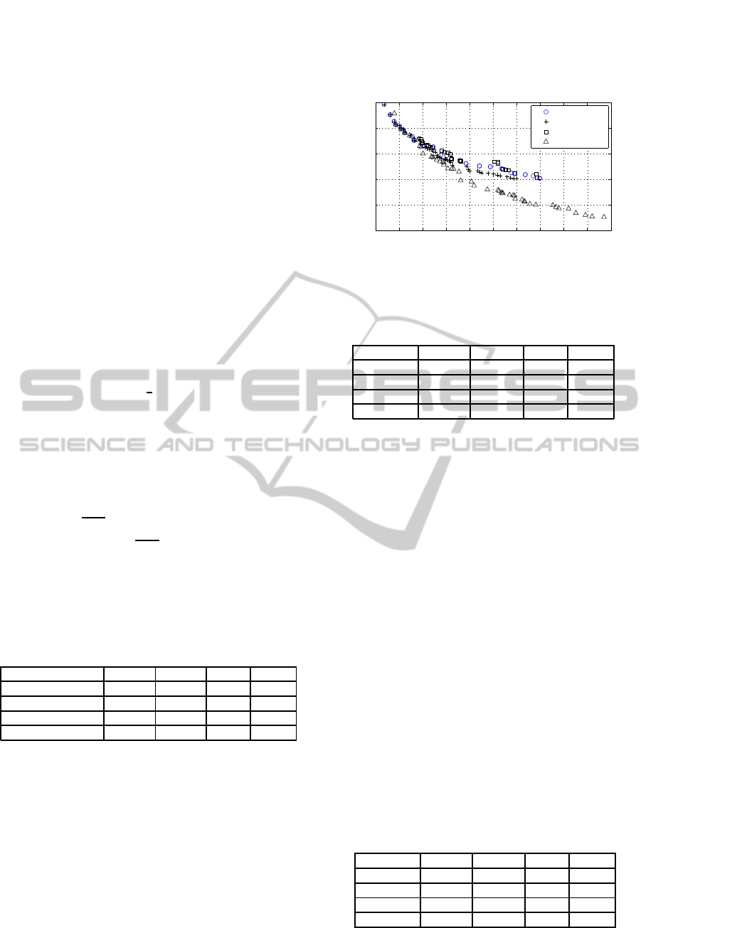
4.2 Case 1 Results

Here, we present the results obtained for case study

1. The problem data is provided in Appendix A. The

BRKGA has the most widely spread front, as it can be

seen in Figure 2, and the average values of the cover-

age metric measure (Zitzler and Thiele, 1999), over

10 optimization runs, as shown in Table 2. We can

oberve that the nondominated solutions of BRKGA

covers relatively higher percentages of the other solu-

tions.

On the one hand, as can be seen in Table 2, on

average the nondominated set achieved by BRKGA

6.2 6.3 6.4 6.5 6.6 6.7 6.8 6.9 7 7.1 7.2

x 10

1.9

2.1

2.2

2.3

2.4

x 10

COST($)

CO2(t−CO2)

NSGA

SPEA

NPGA

BRKGA.NSGA

Figure 2: Pareto-optimal fronts obtained from different al-

gorithms in a single run.

Table 2: Percentage of Nondominated Solutions of set B

covered by those in set A.

set A / set B BRKGA NSGA II NPGA SPEA2

BRKGA 67.3 99.5 70.3

NSGA II 13.9 76 8.8

NPGA 0 10.3 0

SPEA2 13.9 61.3 98.8

dominates about 67.3 % of the nondominated solu-

tions found by NSGA II. However, the front obtained

by NSGA II only dominates in less than 13.9 % of

the nondominated solutions produced by BRKGA.

On the other hand, with regard to NPGA, a BRKGA

front dominates on average 99.5% of the correspond-

ing NPGA front, while the nondominated set pro-

duced by NPGA never dominates the front obtained

by BRKGA. Finally, the nondominated set achivied

by BRKGA dominates about 70.3% of the nondomi-

nated solutions found by SPEA2 while the front ob-

tained by SPEA2 dominates only in less than 13.9%.

4.3 Case 2 Results

In this section, we provide the results obtained for

case study 2. For problem details see Appendix B

and the reference therein. The BRKGA average val-

ues of the coverage metric measure over 10 optimiza-

tion runs are showed in Table 3. We can oberve that

the nondominated solutions of SPEA2 and BRKGA

covers relatively higher percentages of the other solu-

tions.

Table 3: Percentage of Nondominated Solutions coverages.

set A / set B BRKGA NSGA II NPGA SPEA2

BRKGA 88.5 75 30.3

NSGA II 11 49 4

NPGA 22.3 40 10.8

SPEA2 84.8 98.5 92.5

In Table 3, we can observe that, on average,

the nondominated set achieved by BRKGA domi-

ICORES 2012 - 1st International Conference on Operations Research and Enterprise Systems

7.5 7.6 7.7 7.8 7.9 8 8.1 8.2 8.3 8.4 8.5

x 10

4.5

5.5

6.5

7.5

x 10

Fuel cost (x1000) [monetary units]

NOx concentration (x10000) [mg/Nm

]

NSGA

SPEA

NPGA

BRKGA.NSGA

Figure 3: Pareto-optimal fronts obtained from from differ-

ent algorithms in a single run.

nates 88.5% of the nondominated solutions found

by NSGA II, while the front obtained by NSGA II

dominates less than 11 % of the nondominated solu-

tions produced by BRKGA. Moreover, the BRKGA

front dominates on average 75% of the correspond-

ing NPGA front while the nondominatedset produced

by NPGA dominates less than 22.3 % of the non-

dominated solutions produced by BRKGA. Finally,

SPEA2 front dominates on average 84.8% of the cor-

respondingBRKGA front while the nondominated set

produced by BRKGA dominates 30.3 % of the non-

dominated SPEA2 solutions.

5 CONCLUSIONS

In this paper a new approach is used to ﬁnd Pareto sets

for multiobjective unit commitment problem. The

proposed algorithm combines the biased selection and

biased crossover of the BRKGA approach with non-

dominated sorting procedure and crowded compari-

son operator used in NSGA II technique.

The algorithm maintains a ﬁnite-sized archive of

nondominated solutions which gets iteratively up-

dated in the presence of new solutions based on the

concept of pareto dominance. The multiple Pareto

optimal solutions can be found in one simulation run

such as in other multiobjective techniques.

The proposed approach has been assessed through

a comparative study, for two case study problems,

with other multiobjective optimization techniques.

The best results are obtained for SPEA2 and BRKGA

approachs. The results shows that BRKGA can be

an effective method for producing tradeoff curves.

Tradeoff curves such as those presented here may give

decision makers the capability of making better deci-

sions. Given that the approachs have similar decode

procedures, the improvement in performance is most

likely due to elitism. Elitism also guarantees that no

good solutions are lost.

ACKNOWLEDGEMENTS

The ﬁnancial support by FCT, POCI 2010

and FEDER, through project PTDC/EGE-

GES/099741/2008 is gratefully acknowledged.

REFERENCES

Abido, M. A. (2003a). Environmental/economic power dis-

patch using multiobjective evolutionary algorithms.

IEEE Trans. Power Syst., ‘18:‘1529–1537.

Abido, M. A. (2003b). A niched pareto genetic algorithm

for multiobjective environmental/economic dispatch.

Electr. Power Energy Syst., ‘25:97–105.

Abido, M. A. (2003c). A novel multiobjective evolution-

ary algorithm for environmental/economic power dis-

patch. Electr. Power Syst. Res., ‘65:‘71–81.

Abido, M. A. (2006). Multiobjective evolutionary algo-

rithms for electric power dispatch problem. IEEE

Transactions on Evolutionary Computation, ‘10:315–

329.

Basu, M. (2008). Dynamic economic emission dispatch us-

ing non-dominated sorting genetic algorithm-ii. Elec-

tric Power Energy System, 30:140–149.

Deb, K. and Agrawal, R. B. (1995). Simulated binary

crossover for continuous search space. Complex Sys-

tems, 9:115–148.

Deb, K., Pratab, A., Agarwal, S., and Meyarivan, T. (2002).

A fast and elitist multiobjective genetic algorithm:

Nsga-ii. IEEE Trans. Evol. Comput., 6:182–197.

Gonc¸alves, J. F. and Resende, M. G. C. (2010). Biased

random-key genetic algorithms for combinatorial op-

timization. Journal of Heuristics, 17:487–525.

Granelli, G. P., Montagna, M., Pasini, G. L., and Maran-

nino, P. (1992). Emission constrained dynamic dis-

patch. ‘Electr. Power Syst. Res., ‘24:‘56–62.

Horn, J., Nafpliotis, N., and Goldberg, D. E. (1994). A

niched pareto genetic algorithm for multiobjective op-

timization. In 1st IEEE Conf. Evol. Comput., IEEE

World Congr. Comput. Intell., volume 1, pages 67–72.

Hsiao, Y. T., Chiang, H. D., Liu, C. C., and Chen, Y. L.

(1994). A computer package for optimal multiobjec-

tive var planning in large scale power systems. IEEE

Trans. Power Syst., ‘9:‘668–676.

Roque, L., Fontes, D. B. M. M., and Fontes, F. A. C. C.

(2011). A biased random key genetic algorithm ap-

proach for unit commitment problem. Lecture Notes

in Computer Science, 6630:327–339.

Sawaragi, Y., Nakayama, H., and Tanino, T. (1985). Theory

of multiobjective optimization. Orlando: Academic

Press.

Srinivas, N. and Deb, K. (1994). Multiobjective function

optimization using nondominated sorting genetic al-

gorithms. Evol. Comput., 2:221–248.

Wang, S., Shahidehpour, M., Kirschen, D. S., Mokhtari,

S., and Irissari, G. (1995). Short-term generation

scheduling with transmission and environmental con-

straints using an augmented lagrangian relaxation.

IEEE Trans Power Systems, ‘10:1294–300.

BRKGA ADAPTED TO MULTIOBJECTIVE UNIT COMMITMENT - Solving Pareto Frontier for UC Multiobjective

Problem using BRKGA SPEA2 NPGA and NSGA II Techniques

Winter, G., Greiner, D., Gonzalez, B., and Galvan, B.

(2003). Economical and environmental electric power

dispatch optimisation. In ‘EUROGEN-2003 Confer-

ence.

Yamashita, D., Niimura, T., Yokoyama, R., and Marmiroli,

M. (2010). Pareto-optimal solutions for trade-off anal-

ysis of c02 vs. cost based on dp unit commitment. In

2010 International Conference on Power System Tech-

nology.

Yamin, H. Y., El-Dwairi, Q., and Shaihidehpour, S. M.

(2007). A new approach for genco proﬁt based unit

commitment in day-ahead competitive electricity mar-

kets considering reserve uncertainty. Int J Elec Power

Energy Systems, 29:609–16.

Zitzler, E., Laumanns, M., and Thiele, L. (2001). Spea2:

Improving the strength pareto evolutionary algorithm.

TIK-Rep. 103.

Zitzler, E. and Thiele, L. (1998). An evolutionary algorithm

for multiobjective optimization: The strength pareto

approach. TIK-Rep., 43.

Zitzler, E. and Thiele, L. (1999). Multiobjective evolu-

tionary algorithms: A comparative case study and the

strength pareto approach. IEEE Trans. Evol. Comput.,

3:257–271.

APPENDIX A: DATA OF THE CASE

STUDY 1

For more details see (Sawaragiet al., 1985; Yamashita

et al., 2010).

Table 4: Generation constraints in case study 1.

Unit Ymax

Ymin

min,j

off

min,j

Ramp rate

(MW) (MW) (h) (h) (MW/h)

1 455 150 8 8 250

2 455 150 8 8 250

3 130 20 5 5 80

4 130 20 5 5 80

5 162 25 6 6 100

6 80 20 3 3 80

7 85 25 3 3 85

8 55 10 1 1 55

9 55 10 1 1 55

10 55 10 1 1 55

Table 5: Data fuel costs evaluation in case study 1.

Unit A

startup cost

($/MW

h) ($/MWh) ($/h) ($)

1 0.000528 17.809 1100 4950

2 0.000341 18.986 1067 5500

3 0.0022 18.26 770 605

4 0.002321 18.15 748 616

5 0.004378 21.67 495 990

6 0.007832 24.486 407 187

7 0.000869 30.514 528 286

8 0.004543 28.512 726 33

9 0.002442 29.997 731.5 33

10 0.001903 30.569 737 33

Table 6: Data fuel costs evaluation in case study 1.

Unit a

startupCO

(t −CO

/MW

h) (t−CO

//MWh) (t −CO

/h) (t −CO

)

1 2.240E-05 0.7557 46.677 210.0

2 1.446E-05 0.8056 45.276 233.3

3 9.335E-05 0.7748 32.674 25.67

4 9.848E-05 0.7701 31.740 26.13

5 3.197E-05 0.1582 3.6157 7.231

6 5.720E-05 0.1788 2.9729 1.365

7 7.282E-05 0.2557 4.4248 2.396

8 3.807E-05 0.2389 6.0841 0.2765

9 2.046E-05 0.2513 6.1302 0.2765

10 1.594E-05 0.2561 6.1763 0.2765

Table 7: Load demand (MW) in case study 1.

Hour Load demand (MW) Hour Load demand (MW)

1 700 13 1400

2 750 14 1300

3 850 15 1200

4 950 16 1050

5 1000 17 1000

6 1100 18 1100

7 1372 19 1200

8 1314 20 1400

9 1271 21 1300

10 1400 22 1100

11 1450 23 900

12 1500 24 800

APPENDIX B: DATA OF THE CASE

STUDY 2.

For more details see (Winter et al., 2003).

Table 8: Data fuel costs evaluation in case study 2.

Unit Ymax

min,j

off

min,j

(MW) (h) (h) (h) (m.u./MW

) (m.u./MW) (m.u.)

1 520 8 4 -5 0.0085 19.566 4437.2

2 320 5 2 -6 0.0050 20.927 1044.20

3 280 5 2 3 0.0253 18.995 1236.9

4 200 5 2 -3 0.0091 23.107 416.58

5 150 5 3 -7 0.0106 20.765 485.69

6 150 4 2 3 0.0116 22.251 300.86

7 120 4 2 5 0.0212 15.031 315.44

8 100 4 2 1 0.0254 15.031 262.87

9 80 3 1 -1 0.0356 10.375 222.16

10 60 3 1 -1 0.0454 9.9214 159.33

Table 9: Start-up costs, shut down costs and NO

emissions

coefﬁcients in case study 2.

Unit a

(m.u.) (m.u.) (m.u.) (m.u.)

1 267 34.75 0.09 75 -0.245 154.16 -1154.6

2 187 38.62 0.13 70 -0.002 16.414 -691.1

3 176 27.57 0.15 42 -0.069 36.931 -1626

4 227 26.64 0.11 62 0.1313 -20.77 1885.6

5 113 18.64 0.18 29 -0.005 16.287 -321.4

6 282 45.48 0.09 49 0.1686 -20.0 1361.8

7 94 10.65 0.18 32 0.016 1.7774 276.59

8 114 22.57 0.20 40 0.0193 1.7774 230.49

9 101 20.59 0.20 25 -1.793 246.71 -2636

10 85 20.59 0.20 15 -2.286 235.92 -1890

Table 10: Load demand (MW) in case study 2.

Hour Load demand Hour Load demand

(MW) (MW)

1 1459 13 1154

2 1372 14 1138

3 1299 15 1124

4 1280 16 1095

5 1271 17 1066

6 1314 18 1037

7 1372 19 993

8 1314 20 978

9 1271 21 963

10 1242 22 1022

11 1197 23 1081

12 1182 24 1459

ICORES 2012 - 1st International Conference on Operations Research and Enterprise Systems