SPARSE QUASI-NEWTON OPTIMIZATION FOR

SEMI-SUPERVISED SUPPORT VECTOR MACHINES

Fabian Gieseke

, Antti Airola

, Tapio Pahikkala

and Oliver Kramer

Computer Science Department, Carl von Ossietzky Universit

at Oldenburg, 26111 Oldenburg, Germany

Turku Centre for Computer Science, Department of Information Technology, University of Turku, 20520 Turku, Finland

Keywords:

Semi-supervised support vector machines, Non-convex optimization, Quasi-Newton methods, Sparse data,

Nystr

om approximation.

Abstract:

In real-world scenarios, labeled data is often rare while unlabeled data can be obtained in huge quantities.

A current research direction in machine learning is the concept of semi-supervised support vector machines.

This type of binary classiﬁcation approach aims at taking the additional information provided by unlabeled

patterns into account to reveal more information about the structure of the data and, hence, to yield models

with a better classiﬁcation performance. However, generating these semi-supervised models requires solving

difﬁcult optimization tasks. In this work, we present a simple but effective approach to address the induced

optimization task, which is based on a special instance of the quasi-Newton family of optimization schemes.

The resulting framework can be implemented easily using black box optimization engines and yields excel-

lent classiﬁcation and runtime results on both artiﬁcial and real-world data sets that are superior (or at least

competitive) to the ones obtained by competing state-of-the-art methods.

1 INTRODUCTION

One of the most important machine learning tasks

is classiﬁcation. If sufﬁcient labeled training data is

given, there exists a variety of techniques like the

k-nearest neighbor-classiﬁer or support vector ma-

chines (SVMs) (Hastie et al., 2009; Steinwart and

Christmann, 2008) to address such a task. However,

labeled data is often rare in real-world applications.

One active research ﬁeld in machine learning is semi-

supervised learning (Chapelle et al., 2006b; Zhu and

Goldberg, 2009). In contrast to supervised methods,

the latter class of techniques takes both labeled and

unlabeled data into account to construct appropriate

models. A well-known concept in this ﬁeld are semi-

supervised support vector machines (S

VMs) (Ben-

nett and Demiriz, 1999; Joachims, 1999; Vapnik and

Sterin, 1977) which depict the direct extension of sup-

port vector machines to semi-supervised learning sce-

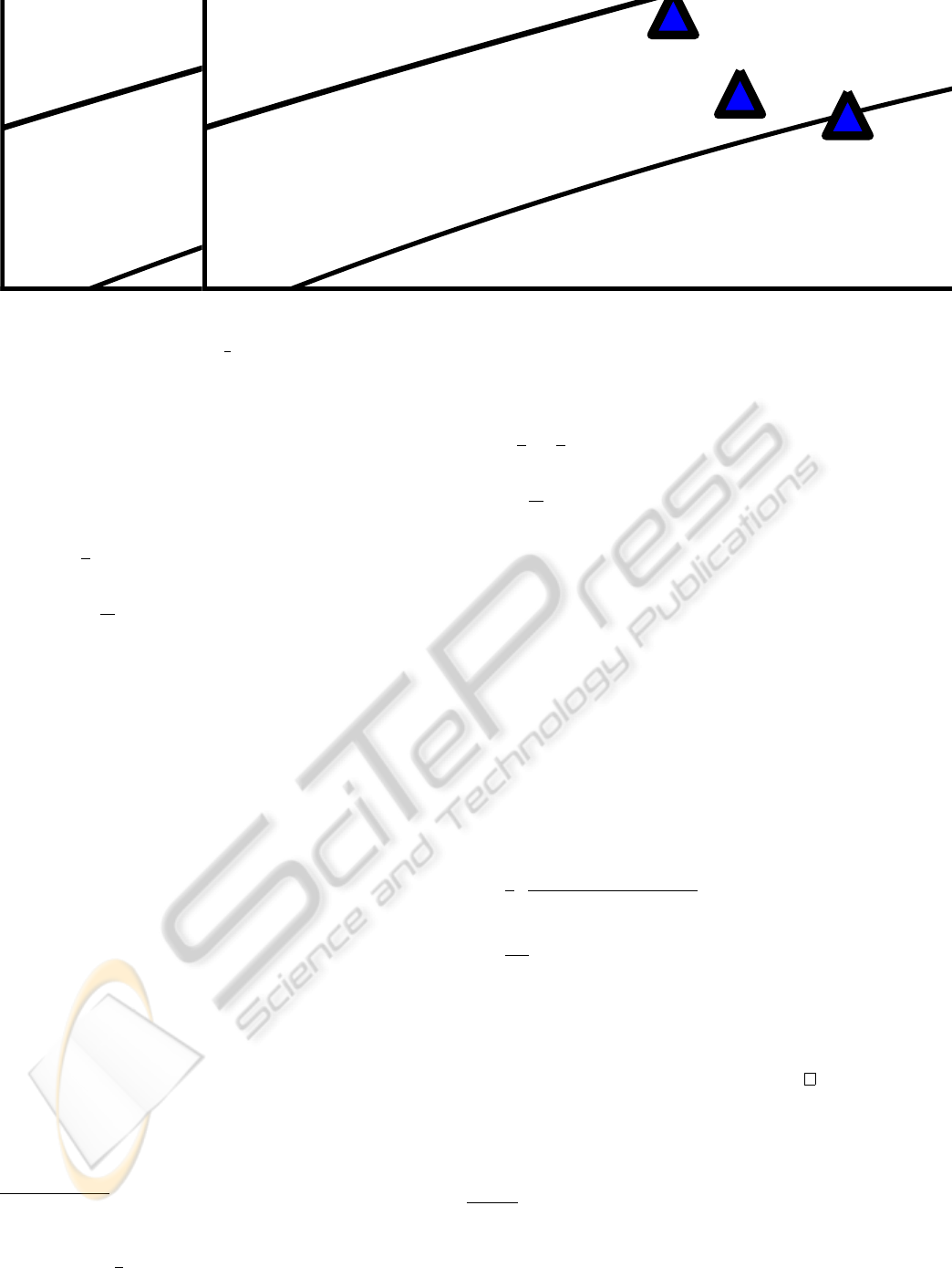
narios. The key idea is depicted in Figure 1: The

aim of a standard support vector machine consists

in ﬁnding a hyperplane which separates both classes

well such that the margin is maximized. It is obvi-

ous that, in case of lack of labeled data, suboptimal

models might be obtained. Its semi-supervised vari-

ant aims at taking the unlabeled patterns into account

by searching for a partition (of these patterns into two

classes) such that a subsequent application of a (mod-

iﬁed) support vector machine leads to the best result.

1.1 Related Work

The original problem formulation of semi-supervised

support vector machines was given by Vapnik and

Sterin (Vapnik and Sterin, 1977) under the name of

transductive support vector machines. From an opti-

mization point of view, the ﬁrst approaches have been

proposed in the late nineties by Joachims (Joachims,

1999) and Bennet and Demiriz (Bennett and Demiriz,

1999). In general, there exist two lines of research,

namely (a) combinatorial and (b) continuous opti-

mization schemes. The naive brute-force approach

(which tests every possible partition), for instance, is

among the combinatorial schemes since it aims at di-

rectly ﬁnding a good assignment for the unknown la-

bels. The continuous optimization perspective (see

below) leads to a real-valued but non-convex task.

For both research directions, a variety of different

techniques has been proposed in recent years that are

based on semi-deﬁnite programming (Bie and Cris-

tianini, 2004; Xu and Schuurmans, 2005), the contin-

uation method (Chapelle et al., 2006a), deterministic

Gieseke F., Airola A., Pahikkala T. and Kramer O. (2012).

SPARSE QUASI-NEWTON OPTIMIZATION FOR SEMI-SUPERVISED SUPPORT VECTOR MACHINES.

In Proceedings of the 1st International Conference on Pattern Recognition Applications and Methods, pages 45-54

DOI: 10.5220/0003755300450054

 SciTePress

(a) SVM (b) S

Figure 1: The concepts of support vector machines and their

extension to semi-supervised learning settings. Labeled pat-

terns are depicted as red squares and blue triangles and un-

labeled patterns as black points, respectively.

annealing (Sindhwani et al., 2006), the (constrained)

concave-convex procedure (Collobert et al., 2006;

Fung and Mangasarian, 2001; Zhao et al., 2008), and

other strategies (Adankon et al., 2009; Chapelle and

Zien, 2005; Mierswa, 2009; Sindhwani and Keerthi,

2006; Zhang et al., 2009). A related approach, also

based on a quasi-Newton framework, is proposed by

Reddy et al. (Reddy et al., 2010); however, they do

not consider differentiable surrogates and therefore

apply more complicated subgradient methods. Many

other approaches exist, and we refer to Chapelle et

al. (Chapelle et al., 2006b; Chapelle et al., 2008) and

Zhu et al. (Zhu and Goldberg, 2009) for comprehen-

sive surveys.

1.2 Notations

We use [m] to denote the set {1, ..., m}. Given a vec-

tor y ∈ R

, we use y

to denote its i-th coordinate.

Further, the set of all m × n matrices with real coefﬁ-

cients is denoted by R

m×n

. Given a matrix M ∈ R

m×n

we denote the element in the i-th row and j-th col-

umn by [M]

i, j

. For two sets R = {i

,. .. ,i

} ⊆ [m]

and S = {k

,. .. ,k

} ⊆ [n] of indices, we use M

to denote the matrix that contains only the rows and

columns of M that are indexed by R and S, respec-

tively. Moreover, we set M

R[n]

= M

2 CLASSIFICATION TASK

In supervised scenarios, we are given a training set

= {(x

),. .. ,(x

)} of labeled patterns x

be-

longing to a set X. The general goal of classiﬁ-

cation approaches consists in building good models

which can predict valuable labels for unseen pat-

terns (Hastie et al., 2009). In semi-supervised learn-

ing frameworks, we are additionally given a set T

l+1

,. .. ,x

l+u

} ⊂ X of unlabeled training patterns.

Here, the goal is to improve the quality of the models

by taking both the labeled and the unlabeled part of

the data into account.

2.1 Support Vector Machines

The concept of support vector machines can be seen

as instance of regularization problems of the form

inf

f ∈H

∑

i=1



, f (x

)



+ λ

, (1)

where λ > 0 is a ﬁxed real number, L : Y × R →

[0,∞) is a loss function and

is the squared

norm in a so-called reproducing kernel Hilbert space

H ⊆ R

= { f : X → R} induced by a kernel func-

tion k : X × X → R (Steinwart and Christmann, 2008).

Here, the ﬁrst term measures the loss caused by the

prediction function on the labeled training set and the

second one penalizes complex functions. Plugging in

different loss functions leads to various models; one

of the most popular choices is the hinge loss L(y,t) =

max(0,1 − yt) which leads to the original deﬁnition

of support vector machines (Sch

olkopf et al., 2001;

Steinwart and Christmann, 2008), see Figure 2 (a).

2.2 Semi-supervised SVMs

Given the additional set T

= {x

l+1

,. .. ,x

l+u

} ⊂ X

of unlabeled training patterns, semi-supervised sup-

port vector machines (Bennett and Demiriz, 1999;

Joachims, 1999; Vapnik and Sterin, 1977) aim at ﬁnd-

ing an optimal prediction function for unseen data

based on both the labeled and the unlabeled part of the

data. More precisely, we search for a function f

∗

∈ H

and a labeling vector y

∗

= (y

∗

,. .. ,y

∗

)

∈ {−1,+1}

that are optimal with respect to

minimize

f ∈H ,y∈{−1,+1}

∑

i=1



, f (x

)



(2)

+ λ

∑

i=1



, f (x

l+i

)



+ λ

where λ

,λ > 0 are user-deﬁned parameters. Thus, the

main task consists in ﬁnding the optimal assignment

vector y for the unlabeled part; the combinatorial na-

ture of this task renders the optimization problem dif-

ﬁcult to solve.

2.3 Continuous Optimization

As mentioned above, one can derive an equivalent

continuous optimization task: Using the hinge loss,

The latter formulation does not include a bias term

b ∈ R, which addresses translated data. For complex kernel

functions like the RBF kernel, adding this bias term does

not yield any known advantages, both from a theoretical as

well as practical point of view (Steinwart and Christmann,

2008). For the linear kernel, a regularized bias effect can be

obtained by adding a dimension of ones to the input data.

ICPRAM 2012 - International Conference on Pattern Recognition Applications and Methods

(a) (b)

Figure 2: The hinge loss L(y,t) = max(0, 1 − yt) and its

differentiable surrogate L(y,t) =

log(1 + exp(γ(1 − yt)))

with y = +1 and γ = 20 are shown in Figure (a). The effec-

tive hinge loss function L(t) = max(0,1 − |t|) along with

its differentiable surrogate L(t) = exp(−st

) with s = 3 are

shown in Figure (b).

the optimal assignments for the vector y for a ﬁxed

f ∈ H are given by y

= sgn( f (x

)) (Chapelle and

Zien, 2005).

This yields

minimize

f ∈H

∑

i=1

max



0,1 − y

f (x

)



(3)

∑

i=1

max



0,1 − | f (x

l+i



+ λ

Note that the effective loss on the unlabeled pat-

terns penalizes predictions around the origin; thus, the

overall loss increases if the decision function f passes

through these patterns, see Figure 2 (b). By applying

the representer theorem (Sch

olkopf et al., 2001) for

latter task, it follows that an optimal solution f ∈ H

is of the form

f (·) =

∑

i=1

k(x

,·) +

∑

i=1

k(x

l+i

,·) (4)

with coefﬁcients c = (c

,. .. ,c

)

∈ R

l+u

Thus, one gets a continuous optimization task which

consists in ﬁnding the optimal coefﬁcient vector c ∈

with n = l + u. Note that the effective loss renders

the task non-convex and non-differentiable (since the

partial functions are non-differentiable).

3 QUASI-NEWTON SCHEME

We will consider a special instance of the quasi-

Newton optimization framework (Nocedal and

Wright, 2000). Besides the objective function itself,

methods belonging to this class of schemes only

require the gradient to be supplied.

Note that the latter observation does only hold without

a balance constraint of the form



∑

i=1

max(0,y

) − b



< ε

for small ε > 0 and b

∈ (0,1).

3.1 Differentiable Surrogates

Aiming at the application of the latter type of

schemes, we introduce the following differentiable

surrogate loss functions depicted in Figure 2. Here,

the differentiable replacement for the hinge loss is the

modiﬁed logistic loss (Zhang and Oles, 2001); the re-

placement for the effective loss for the unlabeled part

is a well-known candidate in this ﬁeld (Chapelle and

Zien, 2005). Thus, the new overall surrogate objec-

tive is given by

∑

i=1

log



1 + exp(γ(1 − y

f (x

)))



(5)

∑

i=1

exp(−3( f (x

l+i

))

)

+ λ

∑

i=1

∑

j=1

k(x

)

with f (·) =

∑

p=1

k(x

,·) and using

∑

i=1

∑

j=1

k(x

) (Sch

olkopf et al., 2001). The

next lemma shows that both a function and a gradient

call can be performed efﬁciently.

Lemma 1. For a given c ∈ R

, one can compute both

the objective F

)

time. The overall space consumption is O(n

Proof. The gradient is given by

∇F

with a ∈ R

and











−

exp(γ(1 − f (x

))

1 + exp(γ(1 − f (x

))

· y

for i ≤ l

−

6λ

· exp



−3( f (x

))



· f (x

) for i > l

Since all predictions f (x

),. .. , f (x

) can be com-

puted in O(n

) total time, one can compute the vector

a ∈ R

and therefore the objective and the gradient in

O(n

). The space requirements are dominated by the

kernel matrix K ∈ R

n×n

Note that numerical instabilities might occur when

evaluating exp(γ(1− f (x

)) for a function or a gra-

dient call. However, one can deal with these degen-

eracies in a safe way since log(1 + exp(t)) − t → 0

and

exp(t)

1+exp(t)

− 1 → 0 converge rapidly for t → ∞.

Thus, each function and gradient evaluation can be

performed spending O(n

) time in a numerically sta-

ble manner.

SPARSE QUASI-NEWTON OPTIMIZATION FOR SEMI-SUPERVISED SUPPORT VECTOR MACHINES

Algorithm 1: QN-S

VM.

Require: A labeled training set T

{(x

),. .. ,(x

)}, an unlabeled training

set T

= {x

l+1

,. .. ,x

}, model parameters

,λ, an initial (positive deﬁnite) inverse

Hessian approximation H

, and a sequence

0 < α

< .. . < α

1: Initialize c

via supervised model.

2: for i = 1 to τ do

3: k = 0

4: while termination criteria not fulﬁlled do

5: Compute search direction p

via (7)

6: Update c

k+1

= c

+ β

7: Update H

k+1

via (8)

8: k = k + 1

9: end while

10: c

= c

11: end for

3.2 Quasi-Newton Framework

One of the most popular quasi-Newton schemes is

the Broyden-Fletcher-Goldfarb-Shanno (BFGS) (No-

cedal and Wright, 2000) method, which we will now

sketch in the context of the given task. The overall

algorithmic framework is given in Algorithm 1: The

initial candidate solution is obtained via Equation (5)

while ignoring the (non-convex) unlabeled part (i. e.,

= 0). The inﬂuence of the unlabeled part is then in-

creased gradually via the sequence α

,. .. ,α

For

each parameter α

, a standard BFGS optimization

phase is performed, i.e., a sequence

k+1

= c

+ β

of candidate solutions is generated, where p

is com-

puted via

= −H

∇F

·λ

) (7)

and where the step length β

is computed via line

search. The approximation H

of the inverse Hessian

is then updated via

k+1

= (I − ρ

(I − ρ

) + ρ

(8)

with z

= ∇F

·λ

k+1

) − ∇F

·λ

), s

= c

k+1

− c

and ρ

= (z

)

−1

. New candidate solutions are gen-

erated as long as a convergence criterion is fulﬁlled

(e. g., as long as



∇F

·λ

)



> ε is fulﬁlled for a

small ε > 0 or as long as the number of iterations is

This sequence can be seen as annealing sequence,

which is a common strategy (Joachims, 1999; Sindhwani

et al., 2006) to create easier problem instances at early

stages of the optimization process and to deform these in-

stances to the ﬁnal task throughout the overall execution.

smaller than a used-deﬁned number). As initial ap-

proximation, one usually resorts to H

= γI for γ > 0;

an important property of the update scheme is that it

preserves the positive deﬁniteness of the inverse Hes-

sian approximations (Nocedal and Wright, 2000).

3.3 Computational Speed-ups

Two main computational bottlenecks arise for large-

scale settings: Firstly, the recurrent computation

of the objective and gradient needed by the quasi-

Newton framework is cumbersome. Secondly, the ap-

proximation of the Hessian’s inverse is, in general,

not sparse, which leads to quadratic-time operations

for the quasi-Newton framework itself (Nocedal and

Wright, 2000). In the following, we will show how to

alleviate these two problems.

3.3.1 Limited Memory Quasi-Newton

The non-sparse approximation of the Hessian’s in-

verse leads to a O(n

) time and to a O(n

) space con-

sumption. To reduce these computational costs, we

consider the L-BFGS methods (Nocedal and Wright,

2000), which depicts a memory and time saving vari-

ant of the original BFGS scheme. In a nutshell,

the idea consists in generating the approximations

,. .. only based on the last m  n iterations and

to perform low-rank updates on the ﬂy without storing

the involved matrices explicitly. This leads to an up-

date time of O(mn) for all operations related to the in-

termediate optimization phases (not counting the time

for function and gradient calls). As pointed out by

Nocedal and Wright, small values for m are usually

sufﬁcient in practice (ranging from, e. g., m = 3 to

m = 50). Thus, assuming m to be a relatively small

constant, the operations needed by the optimization

engine essentially scale linearly with the number n of

optimization variables.

3.3.2 Low-dimensional Search Space

It remains to show how to reduce the second bottle-

neck, i. e., the recurrent computation of both the ob-

jective and the gradient. For this sake, one can resort

to the subset of regressors method (Rifkin, 2002) to

reduce these computational costs, i. e., one approxi-

mates the original hypothesis (4) via

f (·) =

∑

k=1

ˆc

k(x

,·), (9)

where R = { j

,. .. , j

} ⊆ {1,. .. ,n} is a subset of in-

dices. Using this approximation scheme leads to a

slightly modiﬁed objective

(

c) for

c ∈ R

, where

ICPRAM 2012 - International Conference on Pattern Recognition Applications and Methods

the predictions f (x

),. .. , f (x

) are replaced by their

corresponding approximations

f (x

),. .. ,

f (x

) in the

objective (5). Similar derivations as for the non-

approximation case show that the gradient ∇

(

c) is

then given as

∇

(

c) = K

a + 2λK

c, (10)

where f has to be replaced by

f in the former deﬁni-

tion of the vector a ∈ R

. It is easy to see that one can

compute both the new objective as well as its gradient

in an efﬁcient kind of way:

Lemma 2. For

c ∈ R

, the approximated objective

(

c) and the gradient ∇

(

c) can be computed in

O(nr) time spending O(nr) space.

Proof. All predictions

f (x

),. .. ,

f (x

) can be com-

puted in O(nr) time for a

c ∈ R

. Given these pre-

dictions, one can compute the modiﬁed vector a ∈ R

in O(n) time. The remaining operations for obtaining

the new objective

(

c) and its gradient ∇

(

c) can

be performed in O(nr + r

) = O(nr) time. The space

consumption, dominated by K

, is O(nr).

Thus, in combination with the L-BFGS scheme de-

picted above, both the runtime as well as the space

consumption are reduced signiﬁcantly. Here, the pa-

rameter r ∈ {1,...,n} determines a trade-off between

the achieved speed-up and the accuracy of the approx-

imation. Another way to obtain considerable speed-

ups can be achieved for the special case of a linear

kernel, which we will describe next.

3.3.3 Linear Kernel and Sparse Data

Assume that we are given patterns in X = R

and

let X ∈ R

n×d

denote the data matrix containing the

training patterns as rows. In case of the linear kernel,

one can write the kernel matrix as K = XX

∈ R

n×n

and can achieve substantial computational savings by

avoiding its explicit construction. This is the case, for

instance, if the data resides in a low-dimensional fea-

ture space (i.e., d  n) or due to the data matrix being

sparse, meaning that it contains only few nonzero en-

tries.

Lemma 3. For a linear kernel with patterns in X =

, one can compute the objective F

dient ∇F

given candidate solution c ∈ R

Proof. Due to the linear kernel, one can compute

Kc = X(X

c) (11)

and thus all predictions f (x

),. .. , f (x

) in O(nd)

time. In the same manner, one can obtain c

Kc and

Ka in O(nd) time (where the vector a ∈ R

can be

computed in O(n) time given the predictions). Thus,

both the objective F

be obtained in O(nd) time. The space requirements

are bounded by the space needed to store the data ma-

trix X ∈ R

n×d

, which is O(nd).

For high-dimensional but sparse data (i. e., if the ma-

trix X ∈ R

n×d

contains only s  nd nonzero entries),

one can further reduce the computational cost in the

following kind of way:

Lemma 4. For a linear kernel with patterns in X =

and data matrix X ∈ R

n×d

with s  nd nonzero

entries, one can compute the objective F

gradient ∇F

given candidate solution c ∈ R

Proof. Without loss of generality, we assume that

s ≥ n − 1 holds. Similar to the derivations above,

one can compute Kc = X(X

c) and therefore the pre-

dictions f (x

),. .. , f (x

) as well as a ∈ R

in O(s)

time using standard sparse matrix multiplication tech-

niques. In the same way, one can compute c

Kc and

Ka in O(s) time. Hence, both the objective F

(c)

and the gradient ∇F

spending O(s) space.

4 EXPERIMENTS

We will now describe the experimental setup and the

outcome of our experimental evaluation.

4.1 Experimental Setup

The runtime analysis are performed on a 3 GHZ Intel

Core

Duo PC running Ubuntu 10.04. We start by

providing details related to the experimental setup.

4.1.1 Implementation Details

Our implementation is based on Python, the

Scipy package (using the L-BFGS implementation

optimize.fmin l bfgs b (Byrd et al., 1995) with

m = 50), and the Numpy package. The function and

gradient evaluations are based on efﬁcient matrix op-

erations provided by the Numpy package. As pointed

out above, a direct implementation of the latter ones

might suffer from numerical instabilities. To avoid

these instabilities, we make use of log(1+ exp(t)) ≈ t

and

exp(t)

1+exp(t)

≈ 1 for t ≥ 500. We denote the resulting

implementation by QN-S

VM.

Note that the term s is sometimes used to denote the

average number of nonzero entries per pattern x

∈ X in the

training set.

SPARSE QUASI-NEWTON OPTIMIZATION FOR SEMI-SUPERVISED SUPPORT VECTOR MACHINES

(a) Gaussian2C (b) Gaussian4C (c) Moons

Figure 3: Distribution of all artiﬁcial data sets (d = 2). The red squares and blue triangles depict the labeled part of the

data; the remaining black points correspond to the unlabeled part. Note that the two Gaussian data sets depict easy learning

instances for d = 2, even given only few labeled patterns. However, the noise present in the data render the induced tasks

difﬁcult to approach in high dimensions (d = 500) in case only few labeled patterns are given (for supervised models).

4.1.2 Data Sets

We consider several artiﬁcial and real-world data sets,

where the ﬁrst half of each data set is used as train-

ing and the second half as test set. To induce semi-

supervised scenarios, we split each training set into

a labeled and an unlabeled part and use different ra-

tios for the particular setting (where l, u, t denotes

the number of labeled, unlabeled, and test patterns,

respectively).

Artiﬁcial Data Sets. The ﬁrst artiﬁcial data set

is composed of two Gaussian clusters; to gen-

erate it, we draw n/2 points from each of two

multivariate Gaussian distributions X

∼ N (m

,I),

where m

= (−2.5,0.0,. .. ,0.0) ∈ R

and m

(+2.5,0.0, .. ., 0.0) ∈ R

. The class label of a point

corresponds to the distribution it was drawn from,

see Figure 3 (a). If not noted otherwise, we use

n = 500 and d = 500 and denote the induced data set

by Gaussian2C. The second artiﬁcial data set aims

at generating a (possibly) misleading structure: Here,

we draw n/4 points from each of four multivariate

Gaussian distributions X

∼ N (m

,I), where

= (−2.5,−5.0, 0.0,...,0.0) ∈ R

= (−2.5,+5.0, 0.0,...,0.0) ∈ R

= (+2.5,−5.0, 0.0,...,0.0) ∈ R

= (+2.5,+5.0, 0.0,...,0.0) ∈ R

see Figure 3 (b). The points drawn from the ﬁrst two

distributions belong to the ﬁrst class and the remain-

ing one to the second class. Again, we ﬁx n = 500

and d = 500 and denote the corresponding data set

by Gaussian4C. Finally, we consider the well-known

two-dimensional Moons data set with n = 500 points,

see Figure 3 (c).

Real-world Data Sets. In addition to these artiﬁ-

cial data sets, we consider several real-world data

sets including the COIL (Nene et al., 1996) and the

USPS (Hastie et al., 2009) data sets (consisting of both

the training and test set of the original data set). For

the COIL data set, we reduce the input dimensions

of each image from 128 × 128 to 20 × 20 and use

COIL(i,j) to denote the binary classiﬁcation task in-

duced by the objects i and j out of the available 20

objects (using the ordering given in the data set). A

similar notation is used for the binary classiﬁcation

tasks induced by the 10 classes present in the USPS

data set. For both the COIL and the USPS data set, we

rescaled all pixels such that the resulting values lie be-

tween 0.0 and 1.0. Further, we focus on those pairs of

objects/digits which are difﬁcult to separate. Finally,

we consider the Newsgroup20 and the TEXT data set.

Let latter one is composed of the mac and mswindows

classes of the Newsgroup20 data set (Chapelle and

Zien, 2005).

4.1.3 Model Selection

In semi-supervised settings, model selection can be

unreliable due to the lack of labeled data and is

widely considered to be an open issue (Chapelle et al.,

2006b). Due to this model selection problem, we

consider two scenarios to select (non-ﬁxed) parame-

ters. The ﬁrst one is a non-realistic scenario where

we make use of the test set to evaluate the model

performance.

The second one is a realistic scenario

where only the labels of the labeled part of the train-

ing set are used for model evaluation (via 5-fold cross-

validation). The reason for the non-realistic scenario

is the following: By making use of the test set (with a

large amount of labels), we can ﬁrst evaluate the ﬂex-

ibility of the model, i.e., we can ﬁrst investigate if the

model is in principle capable of adapting to the inher-

ent structure of the data while ignoring the (possible)

problems caused by small validation sets.

In both scenarios, we ﬁrst tune the non-ﬁxed pa-

rameters via grid search and subsequently retrain

the ﬁnal model on the training set with the best

This setup is often considered in related evalua-

tions (Chapelle et al., 2006b).

ICPRAM 2012 - International Conference on Pattern Recognition Applications and Methods

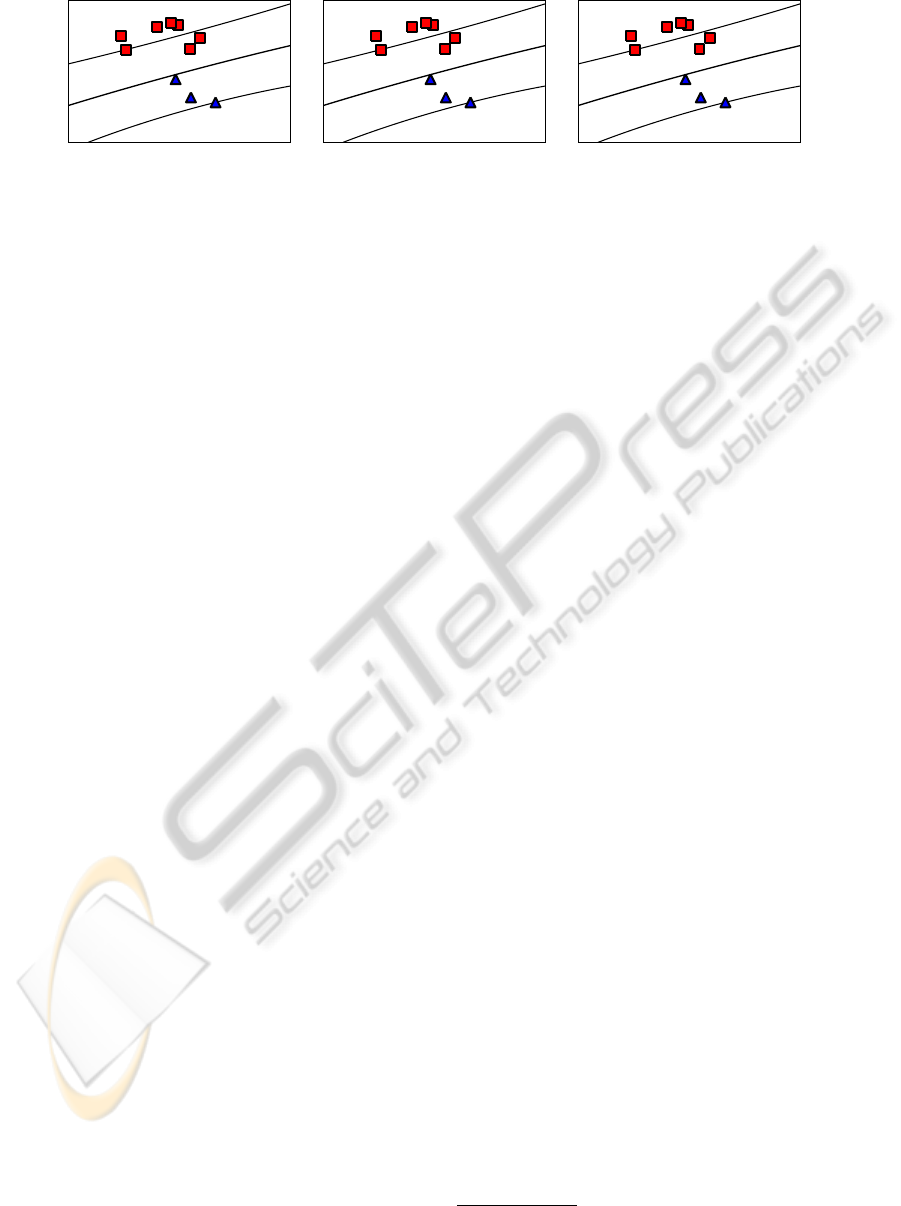
(a) 14.9 ± 8.6 (b) 15.0 ± 9.1 (c) 16.0 ± 10.0

(d) 5.0 ± 6.9 (e) 5.6 ± 7.4 (f) 6.7 ± 8.5

(g) 0.0 ± 0.0 (h) 1.2 ± 2.5 (i) 2.6 ± 2.3

Figure 4: The large red squares and blue triangles depict the labeled data; the small black dots the unlabeled data. Further,

the smaller red squares and blue triangles depict the partition of the unlabeled patterns computed by the semi-supervised

approach. Clearly, the LIBSVM implementation (top row) is not able to generate appropriate models due to the lack of labeled

data. Both the UniverSVM (middle row) and the QN-S

VM approach (bottom row) can successfully incorporate the unlabeled

data, whereas the performance gain is higher for the latter scheme. The average errors (with one standard deviation) on the

test sets over 10 random partitions are reported.

performing set of parameters. As similarity mea-

sures we consider a linear k(x

) = hx

i and

a radial basis function (RBF) kernel k(x

) =

exp(−(2σ

)

−1



− x



) with kernel width σ. To

select the kernel width σ for the RBF kernel, we con-

sider the set {0.01s, 0.1s,1s, 10s,100s} of possible as-

signments, where the value s is a rough estimate of

the maximum distance between any pair of samples.

. The cost parameters λ and λ

are tuned on a small

grid (λ, λ

) ∈ {2

−10

,. .. ,2

} × {0.01,1, 100} of pos-

sible parameters. Further, a short sequence of anneal-

ing steps is used (α

= 0.01,α

= 0.1,α

= 1.0).

4.1.4 Competing Approaches

We use the LIBSVM (Chang and Lin, 2001) as

supervised competitor with C ∈ {2

−10

,. .. ,2

As semi-supervised competitor, we consider the

UniverSVM approach (Collobert et al., 2006). Again,

we perform grid search for tuning the involved param-

eters ((C,C

∗

) ∈ {2

−10

,. .. ,2

} × {

0.01

1.0

100.0

}).

The ratio between the two classes is provided to the

algorithm via the -w option. Except for the option

s =

∑

k=1

(max([x

]

,...,[x

]

) − min([x

]

,...,[x

]

))

-S option (which we set to −0.3), the default val-

ues for the remaining parameters are used. We se-

lected the UniverSVM approach since it seems to be

the strongest semi-supervised competitor (with pub-

licly available code) both with respect to the running

time and classiﬁcation performance. Further, the cor-

responding algorithmic framework is quite similar to

the one proposed in this work, i.e, surrogate loss func-

tions (ramp loss) along with a continuous local search

scheme (concave-convex procedure) are employed.

4.2 Experimental Results

We will now depict the outcome of several experi-

ments demonstrating the potential of our approach.

A detailed comparison of the UniverSVM approach

with other semi-supervised optimization schemes (like the

TSVM approach (Joachims, 1999)) has been conducted by

Collobert et al. (Collobert et al., 2006). Their results in-

dicate the superior performance of UniverSVM compared

to related methods. For the sake of exposition, we will

therefore focus on a comparison of our approach with

UniverSVM.

SPARSE QUASI-NEWTON OPTIMIZATION FOR SEMI-SUPERVISED SUPPORT VECTOR MACHINES

10 20 30 40 50 60 70 80

Test Error (%)

Amount of Labeled Data (%)

LIBSVM

QN−S

(a)

10 20 30 40 50 60 70 80

Test Error (%)

Amount of Labeled Data (%)

LIBSVM

QN−S

(b)

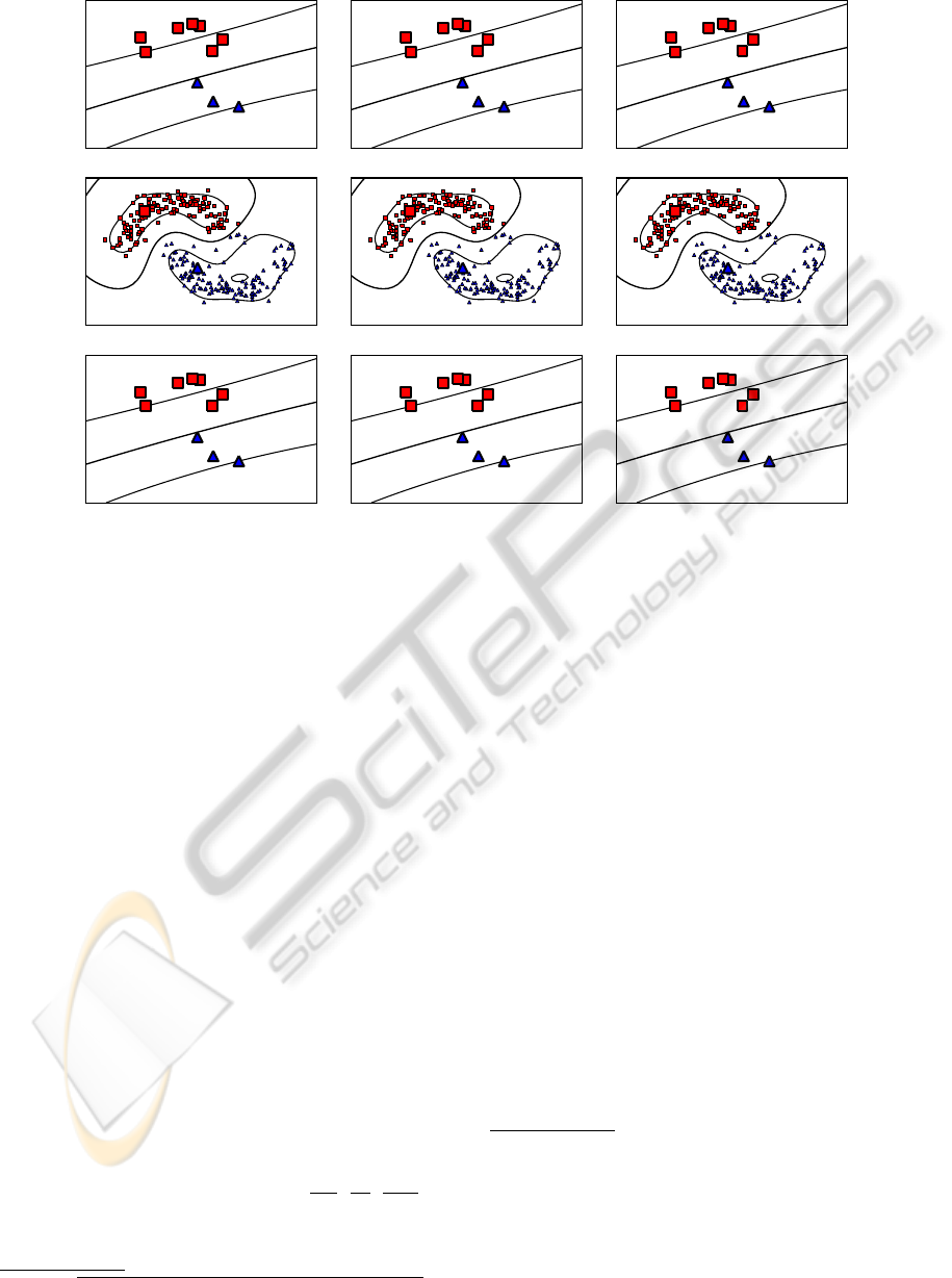
Figure 5: The QN-S

VM approach can incorporate unlabeled data to improve the performance, see Figure (a). However,

sufﬁcient unlabeled data is needed as well to reveal sufﬁcient information about the structure of the data, see Figure (b).

50 150 300 400 500

Runtime (seconds)

Unlabeled Patterns

QN−S

UniverSVM

(a) Gaussian2C

100 300 500 700 1000

Runtime (seconds)

Unlabeled Patterns

QN−S

UniverSVM

(b) USPS(8,0)

100 300 500 800

Runtime (seconds)

Unlabeled Patterns

QN−S

UniverSVM

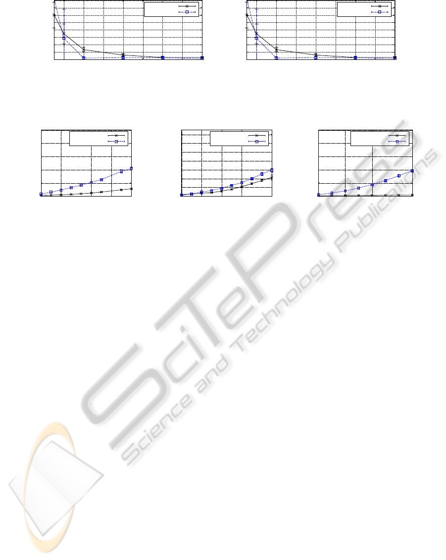
Figure 6: Runtimes for both QN-S

VM and UniverSVM evaluated on three data sets.

4.2.1 Model Flexibility

The well-known Moons data set is said to be a dif-

ﬁcult training instance for semi-supervised support

vector machines due to its non-linear structure. In

Figure 4, the results for the LIBSVM (top row), the

UniverSVM (middle row), and the QN-S

VM imple-

mentation (bottom row) are shown given slightly

varying distributions (using the RBF kernel). To se-

lect the model parameters, we make use of the test

set (non-realistic scenario). For all ﬁgures, the aver-

age test error (with one standard deviation) over 10

random partitions into labeled, unlabeled, and test

patterns, is given. It can be clearly seen that the

supervised approach is not able to generate reason-

able models. Further, the semi-supervised approaches

can successfully incorporate the additional informa-

tion provided by the unlabeled data, whereas the

QN-S

VM scheme seems to perform better on this par-

ticular data set instances.

4.2.2 Amount of Data

As motivated above, sufﬁcient labeled data is essen-

tial for supervised learning approaches to yield rea-

sonable models. For semi-supervised approaches,

the amount of unlabeled data used for training is an

important issue as well. To analyze how much la-

beled and unlabeled data is needed for our approach,

we consider the Gaussian4C data set and vary the

amount of labeled and unlabeled data. For this ex-

periment, we make use of the non-realistic scenario

and resort to the LIBSVM implementation as baseline.

First, we vary the amount of labeled data from 5%

to 80% with respect to (the size of) the training set;

the remaining part the training set is used as unla-

beled data. In Figure 5 (a), the result of this exper-

iment is shown: Given more than 20% labeled data,

the semi-supervised approach performs clearly bet-

ter. Now, we ﬁx the amount of labeled data to 20%

and vary the amount of unlabeled data from 5% to

80% with respect to (the size of) the training set, see

Figure 5 (b). Clearly, the semi-supervised approach

needs sufﬁcient unlabeled data to yield appropriate

models in a reliable manner.

4.2.3 Classiﬁcation Performance

We consider both the realistic and the non-realistic

scenario to evaluate the classiﬁcation performance of

our approach. For each data set, we analyze the be-

havior of all competing approach given up to three

amounts of labeled, unlabeled, and test patterns. For

all data sets and for all competing approaches, a lin-

ear kernel is used. In Table 1, the test errors (and

one standard deviations) averaged over 10 random

partitions are given for both scenarios. It can be

clearly seen that, for the non-realistic scenario, the

semi-supervised approaches mostly yield better re-

sults compared to LIBSVM, even if only few labeled

patterns are given. Thus, they can successfully incor-

porate the additional information provided by the un-

labeled data. Due to lack of labeled data for model se-

lection, the results for the realistic scenario are worse

ICPRAM 2012 - International Conference on Pattern Recognition Applications and Methods

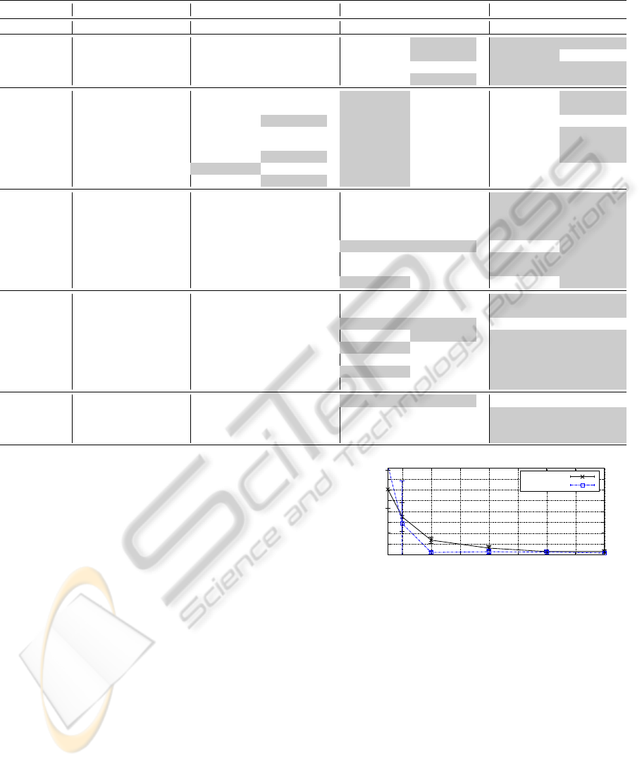
Table 1: Classiﬁcation performances of all competing approaches for both the non-realistic and the realistic scenario. The

best results with respect to the average test errors are highlighted.

Data Set l u t LIBSVM UniverSVM QN-S

non-realistic realistic non-realistic realistic non-realistic realistic

Gaussian2C 25 225 250 13.0 ± 2.9 13.2 ± 2.8 1.0 ± 0.5 1.8 ± 0.9 0.5 ± 0.5 1.8 ± 0.6

Gaussian2C 50 200 250 5.8 ± 2.2 6.3 ± 2.4 1.0 ± 0.4 1.8 ± 0.8 0.5 ± 0.6 2.1 ± 1.0

Gaussian4C 25 225 250 17.4 ± 6.6 20.6 ± 11.5 7.6 ± 12.2 13.3 ± 15.2 6.8 ± 11.9 10.7 ± 13.9

Gaussian4C 50 200 250 6.7 ± 1.5 6.9 ± 1.6 1.6 ± 0.8 2.5 ± 1.5 0.9 ± 0.6 2.5 ± 1.0

COIL(3,6) 14 101 29 13.4 ± 7.0 16.2 ± 7.2 2.8 ± 3.7 16.9 ± 13.9 7.6 ± 9.1 13.1 ± 12.5

COIL(3,6) 28 87 29 3.1 ± 3.3 3.8 ± 4.2 0.3 ± 1.0 5.2 ± 5.8 2.1 ± 3.5 3.1 ± 5.0

COIL(5,9) 14 101 29 13.4 ± 7.0 13.4 ± 7.8 6.9 ± 7.2 19.3 ± 10.9 10.0 ± 8.5 17.9 ± 12.0

COIL(5,9) 28 87 29 3.4 ± 4.1 4.5 ± 5.6 1.4 ± 3.2 7.2 ± 9.1 3.1 ± 5.0 3.8 ± 4.7

COIL(6,19) 14 101 29 12.1 ± 9.8 15.5 ± 13.1 4.5 ± 8.2 21.0 ± 12.0 10.3 ± 10.9 13.4 ± 11.8

COIL(6,19) 28 87 29 3.1 ± 3.3 3.4 ± 3.4 0.7 ± 2.1 4.5 ± 5.1 1.7 ± 3.2 3.4 ± 4.1

COIL(18,19) 14 101 29 6.9 ± 8.0 6.9 ± 8.0 1.0 ± 3.1 7.6 ± 8.8 10.0 ± 9.4 14.1 ± 9.9

COIL(18,19) 28 87 29 1.4 ± 4.1 1.4 ± 4.2 0.0 ± 0.0 5.2 ± 9.7 3.1 ± 5.4 5.9 ± 9.1

USPS(2,5) 16 806 823 9.4 ± 5.1 10.5 ± 4.7 3.2 ± 0.5 9.0 ± 5.6 3.1 ± 0.3 4.7 ± 1.2

USPS(2,5) 32 790 823 4.7 ± 0.7 5.4 ± 0.8 3.2 ± 0.5 5.7 ± 1.8 2.6 ± 0.6 4.0 ± 1.1

USPS(2,7)

17 843 861 4.6 ± 3.0 4.9 ± 2.9 1.5 ± 0.3 6.1 ± 5.3 1.2 ± 0.2 1.5 ± 0.2

USPS(2,7) 34 826 861 2.5 ± 1.0 2.8 ± 1.1 1.4 ± 0.2 3.4 ± 2.4 1.2 ± 0.1 1.5 ± 0.5

USPS(3,8) 15 751 766 12.0 ± 8.2 12.9 ± 8.3 4.8 ± 1.1 8.7 ± 3.9 6.5 ± 7.7 8.7 ± 11.1

USPS(3,8) 30 736 766 6.6 ± 2.1 7.3 ± 2.1 4.0 ± 0.1 7.1 ± 1.8 3.7 ± 1.2 5.5 ± 2.8

USPS(8,0) 22 1, 108 1,131 4.8 ± 1.7 5.0 ± 2.0 1.7 ± 0.7 3.2 ± 2.2 1.4 ± 0.6 2.4 ± 1.5

USPS(8,0) 45 1, 085 1,131 2.7 ± 0.8 3.0 ± 0.9 1.3 ± 0.4 3.3 ± 1.8 1.4 ± 0.7 1.7 ± 0.6

MNIST(1,7) 20 480 500 3.5 ± 1.3 4.2 ± 1.6 2.6 ± 1.0 4.3 ± 2.8 1.8 ± 0.7 2.5 ± 0.9

MNIST(1,7) 50 450 500 2.3 ± 1.0 2.6 ± 1.0 2.2 ± 0.9 3.7 ± 2.5 1.8 ± 0.9 2.3 ± 1.1

MNIST(2,5) 20 480 500 9.3 ± 3.2 10.2 ± 3.1 3.4 ± 0.7 6.3 ± 3.9 4.0 ± 3.1 6.4 ± 3.7

MNIST(2,5) 50 450 500 4.7 ± 1.2 5.8 ± 1.7 3.4 ± 0.7 4.2 ± 1.6 2.4 ± 0.6 4.2 ± 1.3

MNIST(2,7) 20 480 500 6.7 ± 3.7 7.9 ± 4.4 2.9 ± 0.6 8.0 ± 4.7 2.9 ± 1.1 3.9 ± 1.3

MNIST(2,7) 50 450 500 4.2 ± 1.2 5.0 ± 1.5 2.5 ± 0.5 5.1 ± 1.6 2.2 ± 0.4 3.7 ± 2.1

MNIST(3,8) 20 480 500 15.2 ± 4.1 18.8 ± 11.5 8.6 ± 3.3 16.1 ± 3.9 8.6 ± 5.1 12.7 ± 5.9

MNIST(3,8) 50 450 500 8.6 ± 2.5 9.0 ± 2.4 6.3 ± 2.0 9.5 ± 4.1 6.2 ± 2.2 7.5 ± 2.9

TEXT 48 924 974 23.5 ± 6.7 24.8 ± 9.6 6.5 ± 1.0 10.4 ± 2.6 8.2 ± 4.7 21.2 ± 13.8

TEXT 97 876 973 11.4 ± 4.1 11.6 ± 4.1 5.8 ± 0.6 8.5 ± 4.2 5.3 ± 0.9 8.3 ± 2.5

TEXT 194 779 973 7.4 ± 1.3 7.6 ± 1.3 5.2 ± 0.8 6.5 ± 1.5 4.9 ± 0.8 5.4 ± 1.0

TEXT 389 584 973 4.8 ± 0.7 4.8 ± 0.7 4.2 ± 0.6 4.8 ± 0.6 4.0 ± 0.6 4.5 ± 0.6

compared to the non-realistic one. Still, except for the

COIL data sets, the results for QN-S

VM are at least as

good as the ones of LIBSVM.

4.2.4 Computational Considerations

We will ﬁnally focus on the runtime behavior. To

simplify the setup, we ﬁx the model parameters (i. e.,

λ = 1 and λ

= 1) and use a linear kernel.

Medium-scale Scenarios. To give an idea of the

runtime needed to obtain the results provided in Ta-

ble 1, we consider the Gaussian2C, the USPS(8,0)

and the sparse TEXT data set (with l = 25, 22, and

48 labeled patterns, respectively). Further, we vary

the amount of unlabeled patterns as shown in Fig-

ure 6; the average runtime over 10 runs is provided.

The plots indicate a comparable runtime behavior on

the non-sparse data sets. On the sparse text data set,

however, the QN-S

VM is considerably faster; note that

even with 1,000 unlabeled examples, the practical

runtime is less than 0.1 seconds per single execution.

10 20 30 40 50 60 70 80

Test Error (%)

Amount of Labeled Data (%)

LIBSVM

QN−S

Figure 7: Large-Scale experiment.

Large-scale Scenarios. To sketch the applicability

in large-scale settings, we consider the MNIST(1,7)

and vary the size of the training set from 2, 000 to

10,000 patterns. Further, we make use of the kernel

matrix approximation scheme with r = 2, 000 (and

randomly selected basis vectors). The runtime and

the needed function calls are given in Figure 7. As it

can be seen, the runtime is still moderate. Further, it

seems that a constant amount of function calls (being

independent of the size of the training set) is needed.

SPARSE QUASI-NEWTON OPTIMIZATION FOR SEMI-SUPERVISED SUPPORT VECTOR MACHINES

5 CONCLUSIONS

We proposed a quasi-Newton optimization frame-

work for the non-convex task induced by semi-

supervised support vector machines. It seems that

this type of optimization schemes is well suited for

the task at hand since it (a) can be implemented eas-

ily due to its conceptual simplicity and (b) admits di-

rect accelerations for sparse and non-sparse data. The

experiments indicate that the resulting approach can

successfully incorporate unlabeled data, even in real-

istic scenarios where the lack of labeled data compli-

cates the model selection phase.

ACKNOWLEDGEMENTS

This work has been supported in part by funds of

the Deutsche Forschungsgemeinschaft (DFG) (Fabian

Gieseke, grant KR 3695) and by the Academy of

Finland (Tapio Pahikkala, grant 134020). The au-

thors would like to thank the anonymous reviewers

for valuable comments and suggestions.

REFERENCES

Adankon, M., Cheriet, M., and Biem, A. (2009). Semisu-

pervised least squares support vector machine. IEEE

Transactions on Neural Networks, 20(12):1858–1870.

Bennett, K. P. and Demiriz, A. (1999). Semi-supervised

support vector machines. In Adv. in Neural Informa-

tion Proc. Systems 11, pages 368–374. MIT Press.

Bie, T. D. and Cristianini, N. (2004). Convex methods for

transduction. In Adv. in Neural Information Proc. Sys-

tems 16, pages 73–80. MIT Press.

Byrd, R. H., Byrd, R. H., Lu, P., Lu, P., Nocedal, J.,

Nocedal, J., Zhu, C., and Zhu, C. (1995). A lim-

ited memory algorithm for bound constrained opti-

mization. SIAM Journal on Scientiﬁc Computing,

16(5):1190–1208.

Chang, C.-C. and Lin, C.-J. (2001). LIBSVM: a library

for support vector machines. Software available at

http://www.csie.ntu.edu.tw/ cjlin/libsvm.

Chapelle, O., Chi, M., and Zien, A. (2006a). A continuation

method for semi-supervised SVMs. In Proc. Int. Conf.

on Mach. Learn., pages 185–192.

Chapelle, O., Sch

olkopf, B., and Zien, A., editors (2006b).

Semi-Supervised Learning. MIT Press, Cambridge,

MA.

Chapelle, O., Sindhwani, V., and Keerthi, S. S. (2008).

Optimization techniques for semi-supervised support

vector machines. Journal of Mach. Learn. Res.,

9:203–233.

Chapelle, O. and Zien, A. (2005). Semi-supervised classi-

ﬁcation by low density separation. In Proc. Tenth Int.

Workshop on Art. Intell. and Statistics, pages 57–64.

Collobert, R., Sinz, F., Weston, J., and Bottou, L. (2006).

Trading convexity for scalability. In Proc. Int. Conf.

on Mach. Learn., pages 201–208.

Fung, G. and Mangasarian, O. L. (2001). Semi-supervised

support vector machines for unlabeled data classiﬁca-

tion. Optimization Methods and Software, 15:29–44.

Hastie, T., Tibshirani, R., and Friedman, J. (2009). The

Elements of Statistical Learning. Springer.

Joachims, T. (1999). Transductive inference for text classi-

ﬁcation using support vector machines. In Proc. Int.

Conf. on Mach. Learn., pages 200–209.

Mierswa, I. (2009). Non-convex and multi-objective opti-

mization in data mining. PhD thesis, Technische Uni-

versit

at Dortmund.

Nene, S., Nayar, S., and Murase, H. (1996). Columbia ob-

ject image library (coil-100). Technical report.

Nocedal, J. and Wright, S. J. (2000). Numerical Optimiza-

tion. Springer, 1 edition.

Reddy, I. S., Shevade, S., and Murty, M. (2010). A fast

quasi-Newton method for semi-supervised SVM. Pat-

tern Recognition, In Press, Corrected Proof.

Rifkin, R. M. (2002). Everything Old is New Again: A Fresh

Look at Historical Approaches in Machine Learning.

PhD thesis, MIT.

Sch

olkopf, B., Herbrich, R., and Smola, A. J. (2001). A

generalized representer theorem. In Helmbold, D. P.

and Williamson, B., editors, Proc. 14th Annual Conf.

on Computational Learning Theory, pages 416–426.

Sindhwani, V., Keerthi, S., and Chapelle, O. (2006). De-

terministic annealing for semi-supervised kernel ma-

chines. In Proc. Int. Conf. on Mach. Learn., pages

841–848.

Sindhwani, V. and Keerthi, S. S. (2006). Large scale semi-

supervised linear SVMs. In Proc. 29th annual interna-

tional ACM SIGIR conference on Research and devel-

opment in information retrieval, pages 477–484, New

York, NY, USA. ACM.

Steinwart, I. and Christmann, A. (2008). Support Vector

Machines. Springer, New York, NY, USA.

Vapnik, V. and Sterin, A. (1977). On structural risk mini-

mization or overall risk in a problem of pattern recog-

nition. Aut. and Remote Control, 10(3):1495–1503.

Xu, L. and Schuurmans, D. (2005). Unsupervised and semi-

supervised multi-class support vector machines. In

Proc. National Conf. on Art. Intell., pages 904–910.

Zhang, K., Kwok, J. T., and Parvin, B. (2009). Prototype

vector machine for large scale semi-supervised learn-

ing. In Proc. of the Int. Conf. on Mach. Learn., pages

1233–1240.

Zhang, T. and Oles, F. J. (2001). Text categorization based

on regularized linear classiﬁcation methods. Informa-

tion Retrieval, 4:5–31.

Zhao, B., Wang, F., and Zhang, C. (2008). Cuts3vm: A

fast semi-supervised svm algorithm. In Proc. 14th

ACM SIGKDD Int. Conf. on Knowledge Discovery

and Data Mining, pages 830–838.

Zhu, X. and Goldberg, A. B. (2009). Introduction to Semi-

Supervised Learning. Morgan and Claypool.

ICPRAM 2012 - International Conference on Pattern Recognition Applications and Methods