PERFORMANCE EVALUATION OF FEATURE DETECTION FOR

LOCAL OPTICAL FLOW TRACKING

Tobias Senst, Brigitte Unger, Ivo Keller and Thomas Sikora

Communication Systems Group, Technische Universit¨at Berlin, Einsteinufer 17, Berlin, Germany

Keywords:

Feature detector, Feature detection Performance evaluation, Tracking, KLT.

Abstract:

Due to its high computational efﬁciency the Kanade Lucas Tomasi feature tracker is still widely accepted and

a utilized method to compute sparse motion ﬁelds or trajectories in video sequences. This method is made up

of a Good Feature To Track feature detection and a pyramidal Lucas Kanade feature tracking algorithm. It is

well known that the Good Feature To Track takes into account the Aperture Problem, but it does not consider

the Generalized Aperture Problem. In this paper we want to provide an evaluation of a set of alternative

feature detection methods. These methods are taken from feature matching techniques like FAST, SIFT and

MSER. The evaluation is based on the Middlebury dataset and performed by using an improved pyramidal

Lucas Kanade method, called RLOF feature tracker. To compare the results of the feature detector and RLOF

pair, we propose a methodology based on accuracy, efﬁciency and covering measurements.

1 INTRODUCTION

Motion based analysis of a video sequence is an im-

portant topic in computer vision and visual surveil-

lance. The KLT feature tracker (Tomasi and Kanade,

1991) still remains as a widely accepted and utilized

method to compute sparsemotion ﬁelds or trajectories

in video sequences due to its high computational ef-

ﬁciency (Ali and Shah, 2007; Hu et al., 2008; Fradet

et al., 2009). The KLT tracker is based on a GFT

(Good Feature To Track) corner detector (Shi and

Tomasi., 1994) and the Lucas/Kanade local optical

ﬂow method (Lucas and Kanade, 1981).

In the recent past several improvements of the Lu-

cas/Kanade method have been developed: Pyrami-

dal implementation (Bouguet, 2000) was proposed

to estimate large motions, parallelizing using the

GPU (Sinha et al., 2006) increases the runtime perfor-

mance drastically, gain adaptive modiﬁcations (Zach

et al., 2008) extend the robustness against varying il-

luminations and robust norms in association with a

adaptive region size (Senst et al., 2011) improve the

robustness against partial occlusion and non Gaussian

noise. Whilst the tracking by local optical ﬂow has

been improved continually, the feature detecting is

still based on the GFT method. This leads to sev-

eral drawbacks. E.g. the GFT does not consider the

multi scale approach of the pyramidal Lucas/Kanade

implementation. Even the Lucas/Kanade local con-

stant motion constraint is not taken into account by

the GFT algorithm. In the recent decades feature de-

tectors were developed for feature matching methods,

e.g. SIFT (Scale Invariant Feature Transform) (Lowe,

1999), SURF (Speeded Up Robust Features) (Bay

et al., 2008) and MSER (Maximally Stable Extremal

Regions) (Matas et al., 2002). These techniques were

applied e.g. in stereo, SLAM (Simultaneous Local-

ization and Mapping) and image stitching applica-

tions.

In this paper, we investigate the usability of sev-

eral feature detectors related to local optical ﬂow

tracking. The evaluation is based on the Middlebury

dataset (Baker et al., 2009). The dataset provides syn-

thetic and realistic pairs of consecutively captured im-

ages and the optical ﬂow as ground truth for each

pair. We provide metrics for sparse motion estima-

tion. These metrics take into account the accuracy,

efﬁciency and the covering of the sparse motion ﬁeld.

2 FEATURE DETECTION

In this section we brieﬂy introducethe set of evaluated

feature detectors. Most of the detectors are designed

for feature matching, whose requirements differ from

the tracking with local optical ﬂow. Feature matching

methods associate feature points of different images

by extracting descriptors from the detected feature lo-

303

Senst T., Unger B., Keller I. and Sikora T. (2012).

PERFORMANCE EVALUATION OF FEATURE DETECTION FOR LOCAL OPTICAL FLOW TRACKING.

In Proceedings of the 1st International Conference on Pattern Recognition Applications and Methods, pages 303-309

DOI: 10.5220/0003731103030309

 SciTePress

cation. Thus the features provide a limited set of well

localized and individually identiﬁable anchor points.

Important properties are repeatability and invariance

against rotation, translation and scaling (Tuytelaars

and Mikolajczyk, 2008).

The local optical ﬂow estimates the feature motion

by a ﬁrst order Taylor approximation of the bright-

ness constancy constraint equation of a speciﬁed re-

gion (Lucas and Kanade, 1981). Thus it depends on

the appearance of vertical and horizontal derivatives

of the image. This is known as the aperture problem.

In addition it constrains that the speciﬁed region con-

tains one moving pattern. This extends the aperture

problem to the generalized aperture problem (Senst

et al., 2011). As a consequence important properties

of the patterns close to the feature points detected by a

feature detector are cornerness and motion constancy.

Good Features to Track. The GFT method (Shi and

Tomasi., 1994) is designed to detect cornerness pat-

terns. The Gradient matrix G is computed for each

pixel as:

G =

∑

Ω





(1)

with the intensity values I(x,y) of a grayscaled im-

age and the spatial derivatives I

for a speciﬁed

region Ω. The gradient matrix is implemented by

means of integral images for I

, I

and I

. Due to

the use of integral images the computational complex-

ity of the gradient matrix is constant and independent

of the size of Ω. A good feature can be identiﬁed

by the maxima of λ(x,y), the smallest eigenvalue of

G. Thus good features prevent the aperture problem.

Certainly strong corners appear at object boundaries,

where multiple motions are very likely. This leads to

the generalized aperture problem. Post processing is

applied by non-maximal suppression and thresholds

at q · max(λ(x,y)), with q the cornerness quality con-

stant.

Pyramidal Good Features to Track. The PGFT

method is the pyramidal extension of the GFT

method. The pyramidal implementation is done by

up-scaling the region Ω based on integral images.

That is more efﬁcient than down-scaling the image.

For each scale the smallest eigenvalue λ

(x,y) of the

corresponding Gradient matrix is computed. A good

feature can be identiﬁed by the maxima of λ(x, y),

whereby:

λ(x,y) = max

(λ

(x,y)) (2)

is the maximal eigenvalue of each scale.

Feature from Accelerated Segment Test. The

FAST (Rosten and Drummond, 2006) method is de-

signed as runtime efﬁcient corner detector. Corners

are assumed at positions with not self-similar patches.

This is measured by considering a circle, where I

is the intensity from the centre of the circle and I

and I

′

are the intensity values on the diameter line

through the center and at the circle, hence at opposite

positions. Thus a patch is not self-similar if pixels at

the circle look different from the centre. The ﬁlter re-

sponse is performed on a Bresenham circle and given

by:

C = min

− I

)

+ (I

′

− I

)

. (3)

Rosten and Drummond proposed a high-speed test to

ﬁnd the minimum in computationally efﬁcient way.

Scale Invariant Feature Transform. The

SIFT (Lowe, 1999) method provides features

that are translation, rotation and scale invariant. To

achieve this, features are selected at maxima and

minima of a DoG (Difference of Gaussian) function

applied in scale space by building an image pyramid

with resampling between each level. Focusing on

speed the DoG is used to approximate the LoG

(Laplacian of Gaussian). The local maxima or

minima are found by comparing the 8 neighbors

at the same level. These maxima or minima are

compared to the next lowest level of the pyramid.

Speeded Up Robust Features. The SURF (Bay

et al., 2008) are designed with a fast scale space

method using DoB (Difference of Box) ﬁlters as a

very basic Hessian matrix approximation. The Hes-

sian matrix H at each scale is deﬁned as:

H =





(4)

where I

is the convolution of the Gaussian second

order derivative with the image I. The DoB ﬁlters are

implemented by integral images, hence the computa-

tion time is independent of the ﬁlter size. The ﬁlter re-

sponse is deﬁned as the weighted approximated Hes-

sian determinant, where local maxima identify blob

like structures. The scale space is analysed by up-

scaling the box ﬁlter, which is more efﬁcient than

down-scaling the image, followed by a scale space

non-maximum suppression.

STAR. The STAR detector is derived from the Cen-

SurE (Center Surround Extrema) detector (Agrawal

et al., 2008). As well as the SURF the CenSurE is

based on box ﬁlters. While DoB ﬁlters are not invari-

ant to rotation, Agrawal introduced center-surround

ﬁlters that are bi-level. The STAR feature detector

uses a center-surrounded bi-level ﬁlter of two rotated

ICPRAM 2012 - International Conference on Pattern Recognition Applications and Methods

304

squares. The ﬁlter response is computed for seven

scales and each pixel of the image. In contrast to

SIFT and SURF the sample size is constant on each

scale and is leading to a full spatial resolution at every

scale. Post processing steps are done by non-maximal

and line suppression. Features that lie along an edge

or line are detected due to the Gradient matrix, see

Eq. 1.

Maximal Stable Extremal Regions. The MSER de-

tector (Matas et al., 2002) is designed to detect afﬁne

invariant subsets of maximal stable extremal regions.

MSER are detected by consecutivly binarizing an im-

age by a threshold. The threshold is applied from the

maximal image intensity value to its minimal. At each

step a set of regions Φ is computed by connected com-

ponents analysis. The ﬁlter response for each region i

is deﬁned as:

= |Φ

i+∆

\Φ

i−∆

|/|Φ

| (5)

where |... | denotes the cardinality and i ± ∆ the re-

gion at ∆th lower or higher threshold level. The

MSER are identiﬁed by the local minimum of q.

3 FEATURE TRACKING

The motion estimation of the detected features is per-

formed using RLOF (Robust Local Optical Flow)

method (Senst et al., 2011) which is derived from the

pyramidal Lucas/Kanade method (Bouguet, 2000).

Based on the spatial and temporal derivatives of a

speciﬁed region Ω the RLOF computes the feature

motion using a robust regression framework. A ro-

bust redescending composed quadratic norm was in-

troduced to increase the robustness of motion estima-

tion compared to pyramidal Lucas/Kanade method.

To improve the behaviour at motion boundaries an

adaptive region size strategy is applied to decrease Ω.

The region Ω of a feature is decreased until the feature

is trackable or a minimal region size is reached. The

decision of being trackable is done by analysing the

smallest eigenvalue λ, see Section 2, and the residual

error of the motion estimates.

For the experiment the following parameters are

used: a minimal region size of 7 × 7, a maximal

region size of 15 × 15, the robust norm parameters

1/2

= (8,50), 3 levels and maximal 20 iterations.

The RLOF is performed bidirectional, thus incorrect

tracked features could be detect. We identify these

by checking the consistency of forward and backward

ﬂow using a threshold ε

= 1:

||d

I(t)→I(t+1)

+ d

I(t+1)→I(t)

|| < ε

(6)

where I(t) → I(t + 1) denote the forward motion and

I(t + 1) → I(t) the reverse.

4 EVALUATION

METHODOLOGY

The Middlebury dataset (Baker et al., 2009) has be-

come an important benchmark regarding dense opti-

cal ﬂow evaluation. It provides synthetic and realistic

pairs of consecutively captured images. The ground

truth is given by optical ﬂow for each pair. We use

the database to evaluate the sparse optical ﬂow re-

sults of the features found by the respective detector

and tracked with the RLOF. We reﬁne the evaluation

methodology of Baker et al. (Baker et al., 2009) in

terms of accuracy, efﬁciency and covering measures.

For each algorithm and each sequence we record the

the set of detected features, T

⊂ T

the set of

tracked trajectories with ˙x

the endpoint of each tra-

jectory as well as the runtime. The respective ground

truth motion is given by ˙x

the ground truth end-

point of each trajectory.

Accuracy Measures. A basic property is the accu-

racy of the estimated tracks. The most commonly

used measure is the endpoint error (Otte and Nagel,

1994) deﬁned by:

EE( ˙x

) = || ˙x

− ˙x

. (7)

The compact statistic of the EE is often only given by

the averages. Thus the measurement is affected by the

outliers. Baker et al. proposed robust statistics by ap-

plying a set of thresholds to the error measurements.

This report is limited so we decide to use the Median

of endpoint errors (MEE).

Efﬁciency Measures. We measure the feature detec-

tion runtime t

, which describes the computational

complexity of the detection method and the tracking

efﬁciency is deﬁned as:

η =

. (8)

In most cases the computational complexity of fea-

ture tracking is dominant. Therefore the tracking ef-

ﬁciency is an important measurement to trace meth-

ods detecting features which produce small MEE but

a large number of rejected trajectories. Finally the t

denotes the overall detection and tracking runtime.

Covering Measures. Compared with the evaluation

of a dense optical ﬂow method the challenge of com-

paring methods producing sparse motion ﬁelds is not

PERFORMANCE EVALUATION OF FEATURE DETECTION FOR LOCAL OPTICAL FLOW TRACKING

305

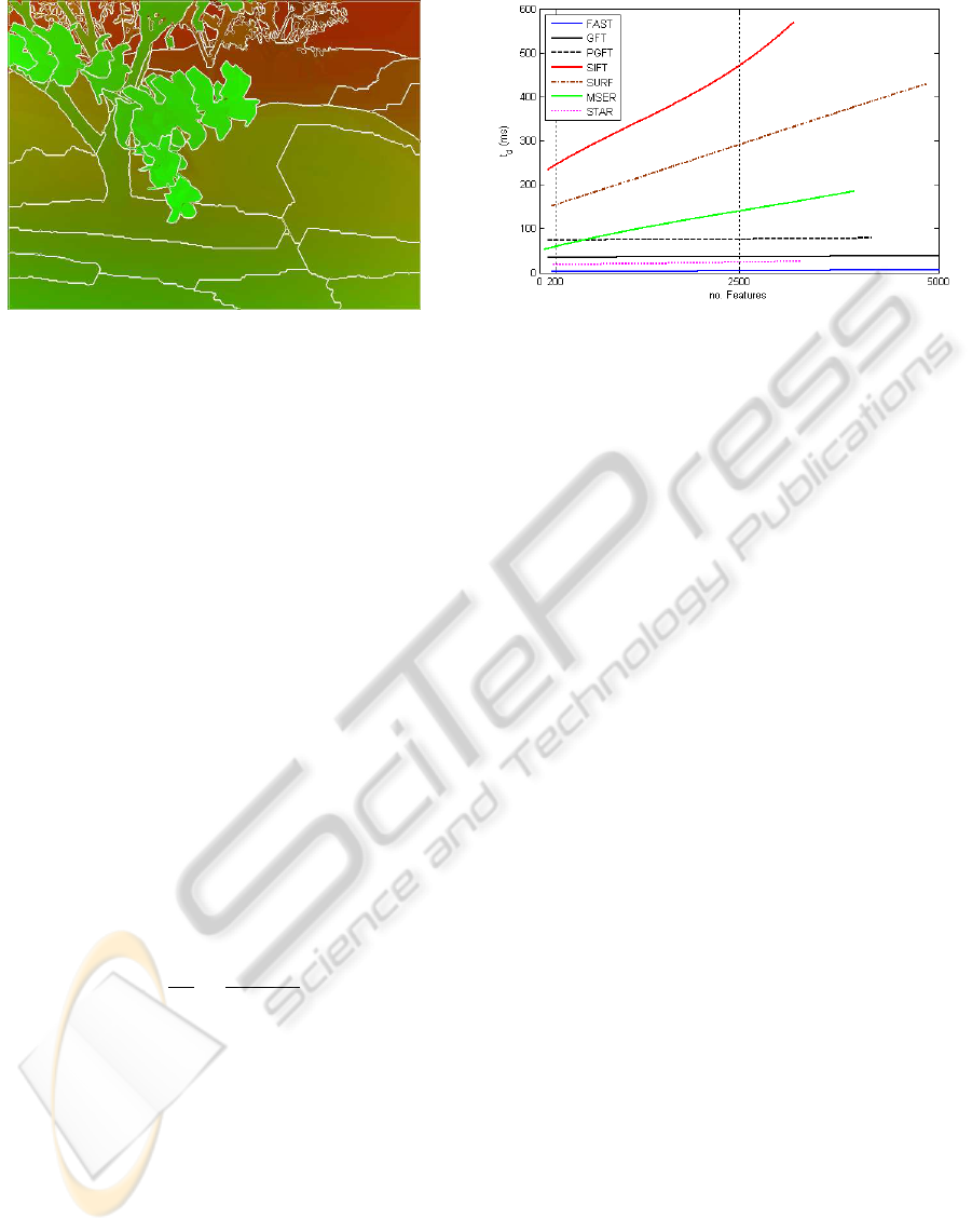
Figure 1: Ground truth optical ﬂow and motion segments of

the Grove2 sequence (The optical ﬂow is shown as color-

code).

only to compare the outliers and the accuracy of the

resulting track, but also to compare whether all the

moving objects are assigned to tracks. In particular

it depends on the application. For example methods

as SLAM (Jonathan and Zhang, 2007) or GME (Tok

et al., 2011) use trajectories of the background. In

these examples it is not critical if the set of trajecto-

ries does not include all foreground objects. But for

applications of motion based image retrieval e.g. ob-

ject segmentation or extraction (Brostow and Cipolla,

2006) all objects have to be covered by trajectories.

The covering measurement ρ is motivated by measur-

ing the ability of the sparse motion ﬁeld to represent

all different moving objects in a scene. At ﬁrst the

ground truth is divided into a set of similar moving

regions C by the color structure code segmentation

method. This algorithm (Rehrmann and Priese, 1997)

is modiﬁed to deal with a 2D motion ﬁeld, see Fig-

ure 1. For each region C the density is computed as

the quotient of the number of tracks |T

⊂ C| located

at C and the area A

of the region. The covering mea-

surement ρ is deﬁned as the mean density.

ρ =

|C|

∑

|C|

⊂ C|

(9)

5 EVALUATION RESULTS

In this paper our goal is to provide a set of baseline

results to allow researchers to get a feel for a feature

detector that has a good performance on their speciﬁc

problem. For this purpose we evaluate the proposed

detection methods at the operating point of around

200 and 2500 feature points. We choose the operating

point of around 200 points to analyze the performance

of the feature detector with few feature points. Partic-

ularly in that case an ideal detector should provide a

Figure 2: Feature detection runtime t

related to the num-

ber of detected features for the Grove3 sequence with VGA

resolution.

high tracking performance, which indicates that the

features are not set to motion boundaries where they

are rejected more likely by the tracker. In contrast

we want to analyze the performance regarding to the

coverage with a denser motion ﬁeld of around 2500

feature points.

The results for all algorithms are shown in Table 1.

The experiments are performed on an AMD Phenom

II X4 960 running at 2.99 GHz. All feature detections

are computed on the CPU. The feature tracking is im-

plemented by the RLOF method running on a Nvidia

GTX 480 graphic device. The results suggest the fol-

lowing conclusions:

FAST. The FAST detector is designed as a high speed

runtime efﬁcient corner detector, which our experi-

ments conﬁrm. For the 640 × 480 Grove3 sequence

the features detection runtime takes only 2 ms. Fig-

ure 2 shows that t

is nearly constant regarding to the

number of detected features. The plain parameteriza-

tion is an additional advantage of this detector. Sum-

marizing the FAST detector is a very fast detector for

a huge set of features with a uniform distribution re-

garding to the moving object.

GFT. The GFT is the third fastest detector in our

benchmark. The runtime t

is constant regarding to

the number of detected features except for a small

growing effort of sorting the features. For a small set

of features the GFT has the best coverage rate at the

Grove2 and Grove3, where the texture is distributed

uniformly. At the Urban2 and Urban3 the detector

achieve the best MEE. However it becomes very in-

efﬁcient when sequences include a large set of strong

edges lying at motion boundaries. These features can-

not be tracked. The GFT is a fast and reliable feature

detector at standard scenarios. But it should be used

with caution at sequences with occlusion and homo-

geneous objects.

ICPRAM 2012 - International Conference on Pattern Recognition Applications and Methods

306

Table 1: Evaluation results for the Middleburry dataset for approximate 200 feature points (left), 2500 feature points (right).

Measurements are t

detection time, t detection and tracking time, η tracking performance, MEE median of endpoint error

and ρ mean feature density per motion segment.

Grove2

Method t

(ms) t (ms) η (%) MEE ρ (%)

GFT 35 98 2.3 0.113 0.42

PGFT 75 138 1.9 0.114 0.42

FAST 2 63 1.5 0.108 0.30

SIFT 240 304 3.9 0.082 0.26

SURF 156 215 5.1 0.116 0.12

STAR 18 76 8.7 0.152 0.22

MSER 63 124 4.8 0.094 0.18

Method t

(ms) t (ms) η (%) MEE ρ (%)

GFT 37 112 2.0 0.069 1.03

PGFT 77 156 1.5 0.073 0.90

FAST 4 73 2.1 0.077 2.10

SIFT 508 588 3.1 0.090 1.04

SURF 280 355 2.3 0.079 0.72

STAR 24 98 2.6 0.082 0.84

MSER 142 215 2.2 0.071 1.62

Grove3

Method t

(ms) t (ms) η (%) MEE ρ (%)

GFT 35 100 6.7 0.168 0.07

PGFT 74 135 8.0 0.165 0.07

FAST 2 64 6.2 0.147 0.03

SIFT 251 318 5.2 0.099 0.06

SURF 151 212 5.4 0.150 0.01

STAR 19 80 9.7 0.134 0.05

MSER 60 123 14.2 0.210 0.02

Method t

(ms) t (ms) η (%) MEE ρ (%)

GFT 37 113 7.7 0.099 0.35

PGFT 77 158 7.3 0.097 0.34

FAST 4 77 9.6 0.138 0.59

SIFT 522 605 9.0 0.129 0.36

SURF 282 358 8.4 0.129 0.40

STAR 24 99 8.4 0.151 0.31

MSER 148 228 9.5 0.110 0.35

Urban2

Method t

(ms) t (ms) η (%) MEE ρ (%)

GFT 35 98 11.8 0.084 0.12

PGFT 75 135 11.8 0.085 0.12

FAST 2 59 14.6 0.104 0.13

SIFT 257 320 4.4 0.103 0.04

SURF 158 219 8.1 0.177 0.19

STAR 19 78 18.6 0.207 0.05

MSER 54 115 16.2 0.154 0.07

Method t

(ms) t (ms) η (%) MEE ρ (%)

GFT 36 117 12.2 0.103 0.64

PGFT 76 159 12.6 0.101 0.59

FAST 5 78 8.6 0.103 1.18

SIFT 506 584 11.8 0.104 0.62

SURF 286 364 10.3 0.126 0.83

STAR 24 99 10.7 0.105 0.63

MSER 104 173 9.8 0.107 0.62

Urban3

Method t

(ms) t (ms) η (%) MEE ρ (%)

GFT 35 101 11.6 0.057 0.12

PGFT 74 134 9.5 0.062 0.19

FAST 2 59 11.3 0.063 0.21

SIFT 272 336 6.6 0.066 0.07

SURF 158 216 10.4 0.107 0.13

STAR 18 78 9.1 0.089 0.22

MSER 51 112 19.7 0.127 0.06

Method t

(ms) t (ms) η (%) MEE ρ (%)

GFT 36 114 13.9 0.089 0.45

PGFT 77 161 12.2 0.085 0.48

FAST 5 76 9.1 0.071 0.82

SIFT 534 616 12.5 0.110 0.54

SURF 300 382 11.5 0.100 0.56

STAR 25 102 10.7 0.081 0.59

MSER 94 158 18.0 0.100 0.34

RubberWhale

Method t

(ms) t (ms) η (%) MEE ρ (%)

GFT 26 77 2.2 0.055 0.06

PGFT 55 106 1.8 0.059 0.07

FAST 1 50 0.5 0.051 0.08

SIFT 183 233 1.1 0.129 0.08

SURF 113 162 4.3 0.180 0.11

STAR 13 62 3.3 0.127 0.10

MSER 51 101 3.0 0.075 0.24

Method t

(ms) t (ms) η (%) MEE ρ (%)

GFT 27 89 3.2 0.057 0.99

PGFT 56 119 3.2 0.057 1.12

FAST 4 63 2.2 0.050 1.25

SIFT 414 476 1.9 0.057 0.78

SURF 237 299 3.3 0.066 1.06

STAR 18 74 2.0 0.057 0.94

MSER 93 148 2.3 0.051 0.54

Venus

Method t

(ms) t (ms) η (%) MEE ρ (%)

GFT 18 65 0.6 0.205 0.16

PGFT 38 82 1.7 0.208 0.17

FAST 1 43 4.5 0.202 0.20

SIFT 128 171 1.5 0.188 0.17

SURF 80 122 2.5 0.185 0.13

STAR 9 52 3.3 0.210 0.21

MSER 33 76 4.8 0.183 0.16

Method t

(ms) t (ms) η (%) MEE ρ (%)

GFT 20 76 6.6 0.225 1.40

PGFT 40 97 7.1 0.235 1.14

FAST 4 57 4.1 0.204 2.28

SIFT 267 319 5.3 0.202 0.83

SURF 218 276 4.9 0.202 1.67

STAR 12 60 4.2 0.227 0.75

MSER 62 108 5.6 0.189 0.67

Hydrangea

Method t

(ms) t (ms) η (%) MEE ρ (%)

GFT 26 80 0.4 0.283 0.42

PGFT 54 106 0.0 0.306 0.42

FAST 1 50 0.5 0.252 0.25

SIFT 177 228 1.7 0.260 0.24

SURF 115 165 3.9 0.261 0.47

STAR 13 62 3.1 0.279 0.33

MSER 40 90 1.5 0.303 0.54

Method t

(ms) t (ms) η (%) MEE ρ (%)

GFT 27 93 4.7 0.091 1.24

PGFT 57 124 3.6 0.090 1.27

FAST 5 68 2.6 0.271 3.30

SIFT 411 484 5.7 0.117 1.51

SURF 257 324 4.6 0.102 1.20

STAR 18 80 3.1 0.105 1.34

MSER 89 151 3.0 0.260 2.70

Dimetrodon

Method t

(ms) t (ms) η (%) MEE ρ (%)

GFT 25 77 0.00 0.049 0.018

PGFT 54 104 0.00 0.057 0.017

FAST 1 49 0.00 0.046 0.017

SIFT 178 230 0.00 0.052 0.019

SURF 113 161 0.00 0.078 0.015

STAR 13 62 0.00 0.051 0.020

MSER 45 96 0.50 0.056 0.017

Method t

(ms) t (ms) η (%) MEE ρ (%)

GFT 27 92 0.5 0.138 0.23

PGFT 56 122 0.6 0.138 0.21

FAST 4 62 0.1 0.058 0.19

SIFT 375 438 1.0 0.085 0.16

SURF 247 310 0.4 0.102 0.21

STAR 18 75 0.6 0.119 0.17

MSER 59 109 0.2 0.059 0.05

PGFT. The PGFT improves the GFT in some se-

quence. E.g. Urban3, RubberWhale and Hydrangea,

there the tracking efﬁciency is decreased and the cov-

erage is increased. However, the beneﬁt results in an

increased detection runtime.

PERFORMANCE EVALUATION OF FEATURE DETECTION FOR LOCAL OPTICAL FLOW TRACKING

307

STAR. Due to the efﬁcient implementation the STAR

method reaches the runtime ranking two. In some

special sequences as Venus or Urban3 it gets good

covering performancewith a low feature set. But gen-

erally the performance of the STAR is below average.

SIFT. As shown in Figure 2 the SIFT detector run-

time depends on the number of features. It is the

slowest of the evaluation. But it shows good perfor-

mance within a low feature set. This method reaches

the best MEE results at Grove2 and Grove3 and the

best tracking performance at the difﬁcult Urban2 and

Urban3. In our experiments the scale space analysis

of the DoG of the SIFT tends to detect less features

at object boundaries. Almost homogeneous regions

are also selected, e.g. the sky of the Grove3 sequence

where tracking is still applicable. Though the set of

objects are not covered uniformly, this results into low

coverage. Summarizing the SIFT detector is a slow

feature detector with a high tracking performance at

sequences with few objects.

SURF. In our experiments the improved runtime per-

formance regarding the SIFT could be conﬁrmed, but

is still high compared to the other detectors. Re-

lated to SIFT the SURF shows some improvements at

large sets of features in terms of tracking performance

and accuracy. But FAST and GFT are still superior at

large feature sets.

MSER. The MSER is the only method based on seg-

mentation instead of ﬁnding features using ﬁrst or

second order derivatives. In our experiments we could

observe that features are less likely detected at ob-

ject boundaries e.g. in the RubberWhale sequence

features are detected in the center of the fence holes

instead of their corners. Considering the generalized

aperture problem this is an important beneﬁt. But it is

not reﬂected in the results of the whole dataset, where

the MSER detector achieve average results. Even at

the Venus sequence it performs the best MEE results.

This sequence is also a challenging sequence for

the GFT because it mainly consists of homogeneous

objects. Most of the cornerness regions are distributed

at the object boundaries. Thus MSER and also the

scale space detector SIFT and SURF achieve good re-

sults. That leads to the conclusion that a region based

or a scale space based approach would be attractive to

improve the GFT method.

6 CONCLUSIONS

In this paper we evaluate different feature detectors in

conjunction with the RLOF local optical ﬂow method.

While the state-of-the-art KLT-Tracker operates with

the GFT detector, our goal is to provide a set of base-

line results for alternative feature detectors to allow

researchers to get a sense of which detector to use

for a good performance on their speciﬁc problem. To

compare the resulting sparse motion ﬁelds we pro-

pose a methodology based on accuracy, efﬁciencyand

coveringmeasurements. The benchmark is performed

on the Middleyburry dataset, which provides a set of

consecutively captured images and the corresponding

dense motion ground truth.

We observethat the efﬁcient performingalgorithm

is the FAST approach. With a runtime of about 3 ms

for a VGA sequence and an overall good performance

for the tracking efﬁciency, median endpoint error and

coverage it outperforms the standard GFT detector.

For standard scenarios i.e. uniform texture distribu-

tion the GFT is a fast and reliable feature detector.

From the results given by the evaluations we conclude

that for speciﬁc sequences, e.g. sequences includ-

ing homogeneous objects, where the texture distribu-

tion concentrates on object boundaries, there is still

room for improvements. Limited advantages shows

the PGFT but also SIFT and MSER shows enhanced

performance under these conditions. Furthermore an

improved GFT method could beneﬁt from the scale

space analysis of the SIFT or the region based ap-

proach of the MSER.

ACKNOWLEDGEMENTS

The research leading to these results has received

funding from the European Community’s FP7 under

grant agreement number 261743 (NoE VideoSense).

REFERENCES

Agrawal, M., Konolige, K., and Blas, M. (2008). Censure:

Center surround extremas for realtime feature detec-

tion and matching. In European Conference on Com-

puter Vision (ECCV 2008), pages 102–115.

Ali, S. and Shah, M. (2007). A lagrangian particle dynam-

ics approach for crowd ﬂowsegmentation and stability

analysis. In Computer Vision and Pattern Recognition

(CVPR 2007), pages 1 –6.

Baker, S., Scharstein, D., Lewis, J., Roth, S., Black, M. J.,

and Szeliski, R. (2009). A database and evaluation

methodology for optical ﬂow. Technical report MSR-

TR-2009-179, Microsoft Research.

Bay, H., Ess, A., Tuytelaars, T., and Gool, L. V. (2008).

Surf: Speeded up robust features. Computer Vision

and Image Understanding, 110(3):346–359.

Bouguet, J.-Y. (2000). Pyramidal implementation of the lu-

cas kanade feature tracker. Technical report, Intel Cor-

poration Microprocessor Research Lab.

ICPRAM 2012 - International Conference on Pattern Recognition Applications and Methods

308

Brostow, G. and Cipolla, R. (2006). Unsupervised bayesian

detection of independent motion in crowds. In Com-

puter Vision and Pattern Recognition (CVPR 2006),

pages 594–601.

Fradet, M., Robert, P., and P´erez, P. (2009). Clustering point

trajectories with various life-spans. In Conference for

Visual Media Production (CVMP 2009), pages 7–14.

Hu, M., Ali, S., and Shah, M. (2008). Detecting global

motion patterns in complex videos. In International

Conference on Pattern Recognition (2008), pages 1 –

Jonathan and Zhang, H. (2007). Quantitative evaluation of

feature extractors for visual slam. In Canadian Con-

ference on Computer and Robot Vision (CRV 2007),

pages 157–164.

Lowe, D. (1999). Object recognition from local scale-

invariant features. In International Conference on

Computer Vision (ICCV 1999), pages 1150–1157.

Lucas, B. D. and Kanade, T. (1981). An iterative image

registration technique with an application to stereo vi-

sion. In International Joint Conference on Artiﬁcial

Intelligence (IJCAI 1981), pages 674–679.

Matas, J., Chum, O., Urban, M., and Pajdla, T. (2002). Ro-

bust wide baseline stereo from maximally stable ex-

tremal regions. In British Machine Vision Conference

(BMVC 2002), pages 384–393.

Otte, M. and Nagel, H.-H. (1994). Optical ﬂow estimation:

Advances and comparisons. In European Conference

on Computer Vision (ECCV 1994), pages 49–60.

Rehrmann, V. and Priese, L. (1997). Fast and robust seg-

mentation of natural color scenes. In Asian Confer-

ence on Computer Vision (ACCV 1997), pages 598–

606.

Rosten, E. and Drummond, T. (2006). Machine learning for

high-speed corner detection. In European Conference

on Computer Vision (ECCV 2006), pages 430–443.

Senst, T., Eiselein, V., Heras Evangelio, R., and Sikora, T.

(2011). Robust modiﬁed L2 local optical ﬂow esti-

mation and feature tracking. In IEEE Workshop on

Motion and Video Computing (WMVC 2011), pages

685–690.

Shi, J. and Tomasi., C. (1994). Good features to track.

In Computer Vision and Pattern Recognition (CVPR

1994), pages 593 –600.

Sinha, S. N., Frahm, J.-M., Pollefeys, M., and Genc, Y.

(2006). Gpu-based video feature tracking and match-

ing. Technical report 06-012, UNC Chapel Hill.

Tok, M., Glantz, A., Krutz, A., and Sikora, T. (2011).

Feature-based global motion estimation using the

helmholtz principle. In International Conference

on Acoustics Speech and Signal Processing (ICASSP

2011), pages 1561–1564.

Tomasi, C. and Kanade, T. (1991). Detection and tracking

of point features. Technical report CMU-CS-91-132,

CMU.

Tuytelaars, T. and Mikolajczyk, K. (2008). Local invariant

feature detectors: a survey. Foundations and Trends

in Computer Vision Graphics Vision., 3:177–280.

Zach, C., Gallup, D., and Frahm, J. (2008). Fast gain-

adaptive klt tracking on the gpu. In Visual Computer

Vision on GPUs workshop (CVGPU 08), pages 1–7.

PERFORMANCE EVALUATION OF FEATURE DETECTION FOR LOCAL OPTICAL FLOW TRACKING

309