A NEW VARIANT OF THE MINORITY GAME

Asset Value Game and Its Extension

Jun Kiniwa

, Takeshi Koide

and Hiroaki Sandoh

Department of Applied Economics, University of Hyogo, Kobe, Japan

Department of Intelligence and Informatics, Konan University, Kobe, Japan

Graduate School of Economics, Osaka University, Toyonaka, Osaka, Japan

Keywords:

Multiagent, Minority game, Mean asset value, Asset value game, Contrarian, Trend-follower.

Abstract:

A minority game (MG) is a non-cooperative iterated game with an odd population of agents who make bids

whether to buy or sell. Based on the framework of MG, several kinds of games have been proposed. However,

the common disadvantage in their characteristics is to neglect past actions. So we present a new variant of

the MG, called an asset value game (AG), in which every agent aims to decrease a mean asset value, that

is, an acquisition cost averaged through the past actions. The AG, however, is too simple to reproduce the

complete market dynamics. So we further consider an improvement of AG, called an extended asset value

game (ExAG), and investigate their features and obtain some results by simulation.

1 INTRODUCTION

Background

A minority game (MG) has been extensively studied

in this decade. It is considered as a model for ﬁnan-

cial markets or other applications in physics. It is a

non-cooperative iterated game with an odd popula-

tion size N of agents who make bids whether to buy

or sell. Since each agent aims to choose the group of

minority population, he is called a contrarian. Every

agent makes a decision at each step based on the pre-

diction of a strategy according to the sequence of the

m most recent outcomes of winners, where m is said

to be the memory size of the agents. Though MG is

a very simple model, it captures some of the complex

macroscopic behavior of the markets.

It is also known that the MG cannot capture large

price drifts such as bubble/crash phenomena, but just

can do the stationary state of the markets. This can be

intuitively explained as follows. Suppose that a group

of buyers can keep a majority for a long time. Then

a group of sellers must continuously win in the bub-

ble phenomenon. However, since every agent wants

to win and thus joins the group of sellers one after

another, it will gain a majority soon. That is, the

group of buyers cannot keep a majority, a contradic-

tion. Thus, it is difﬁcult to simulate the bubble phe-

nomenon by MG.

Related Work

Much work has been done for the purpose of adapt-

ing MG to a real ﬁnancial market. For example, ﬁrst,

several authors investigated the majority game (MJ),

consisting of trend-followers. Marsili (Marsili, 2001)

and Martino et al. (Martino et al., 2003) investigated a

mixed majority-minority gameby varyingthe fraction

of trend-followers. Second, another way is to incor-

porate more realistic mechanism. A grand canonical

minority game (GCMG) (Challet et al., 2001; Ferreira

et al., 2005; Giardina et al., 2001) is considered as one

of the most successful models of a ﬁnancial market.

In the GCMG, a set of agents consist of two groups,

called producers and speculators, and the speculators

are allowed not to trade in addition to buy and sell.

Third, it is also useful to improve the payoff function.

Andersen and Sornette(Andersen and Sornette, 2003)

proposed a different market payoff, called $-game, in

which the timing of strategy evaluation is taken into

consideration. Ferreira and Marsili(Ferreira and Mar-

sili, 2005) compared the behavior of the $-game with

that of the MG/MJ. The difﬁculty of the $-game is

to evaluate its payoff function because we have to

know one step future result. (Kiniwa et al., 2009)

proposed an improved $-game, in which the timing of

evaluation is delayed until the future result is turned

out. Fourth, there are some other kinds of improve-

ment. Liu et al. (Liu et al., 2004) proposed a mod-

Kiniwa J., Koide T. and Sandoh H..

A NEW VARIANT OF THE MINORITY GAME - Asset Value Game and Its Extension.

DOI: 10.5220/0003715800150022

In Proceedings of the 4th International Conference on Agents and Artiﬁcial Intelligence (ICAART-2012), pages 15-22

ISBN: 978-989-8425-96-6

 2012 SCITEPRESS (Science and Technology Publications, Lda.)

iﬁed MG, where agents accumulate scores for their

strategies from the recent several steps. Recent work

by Challet (Challet, 2008) proposed a more sophis-

ticated model using asynchronous holding positions

which are driven by some patterns. Finally, two books

(Challet et al., 2005; Coolen, 2005) comprehensively

described the history of minority games, mathemati-

cal analysis, and their variations. Beyond the frame-

work of MG, efforts to reproduce the real market dy-

namics are continued (Takayasu et al., 1992; Yamada

et al., 2007).

Motivation

The purpose of this paper is also to improve MG by

the thirdly mentioned above. Though the framework

of MG and its variants seem to be reasonable, we

have a basic question — “Do people always make

decisions by using their strategies depending on the

recent history ?” Some people may just take actions

by considering losses and gains. For example, if one

has a company’s stock which has rapidly risen (resp.

fallen), he will sell (resp. not sell) it soon without us-

ing his strategy as illustrated in Figure 1. Such a situa-

tion gives us the idea of an acquisition cost, or a mean

asset value. In the conventional games, like the origi-

nal MG, an agent forgets the past events and makes a

decision by observing only the price up/down within

the memory size

. In our game, however, each agent

evaluates the strategies by whether or not the current

price exceeds his mean asset value. Since the mean

asset value contains all the past events in a sense, he

can increase his net proﬁt by reducing the mean asset

value. We call the game an asset value game, denoted

by AG.

Figure 1: Illustration of our idea.

However, there is still an unsolved problem in AG

that stems from the framework of MG: the payoff

function does not give an action, but just adds points

to desirable strategies. Thus, if the adopted strategy is

Recently, several studies (Araujo and Lamb, 2004;

Araujo and Lamb, 2009) in this direction have been made

from the viewpoint of evolutionary learning.

not desirable, the agent has to wait until the desirable

one gains the highest score. So, there is a time lag be-

tween the rapid change of a price and the adjustment

of an agent’s behavior.

To improve the time lag, we allow each agent

another action that satisﬁes the payoff function with

some probability. If the price rises/falls rapidly and

the difference between the price and agent i’s mean

asset value exceeds some threshold, the agent i may

take the action according to the payoff function (re-

gardless of the strategy). By tuning up the threshold,

etc., we can reproduce the real market dynamics. We

call the variant of AG an extended asset value game,

denoted by ExAG.

Contributions

Our contributions in this paper are summarized as fol-

lows:

• We present a new variant of the MG, called an

asset value game.

• To improve the problem of AG, we further con-

sider an extended AG.

• We investigate the behavior of AG and ExAG in

detail.

The rest of this paper is organized as follows. Sec-

tion 2 states our model, which contains MG, MJ, AG

and ExAG. Section 3 presents an analysis of AG. Sec-

tion 4 describes a simulation model and shows some

experimental results. Finally, Section 5 concludes the

paper.

2 MODELS

In this section, we ﬁrst describe MG and MJ in Sec-

tion 2.1, then the difference between MG and AG in

Section 2.2. Finally, we describe the difference be-

tween AG and ExAG in Section 2.3.

2.1 Previous Model — MG and MJ

At the beginning of the game, each agent i ∈

{1,...,N} is randomly given s strategies R

i,a

for a ∈

{1,.. .,s} . The number of agents, N, is assumed to be

odd in order to break a tie. Any strategy R

i,a

(µ) ∈ R

i,a

maps an m-length binary string µ into a decision −1

or 1, that is,

i,a

: {−1,1}

−→ {−1,1}, (1)

where m is the memory of agents. A history H,

e.g., [−1,1,1, ...], is a sequence of −1 and 1 rep-

resenting a winning decision h(t) for each time step

ICAART 2012 - International Conference on Agents and Artificial Intelligence

t ∈ T = (0, 1, 2,.. .). The winning decision of MG

(resp. MJ) is determined by the minority (resp. ma-

jority) group of −1 or 1. Each strategy R

i,a

(µ) ∈ R

i,a

is given a score U

i,a

(t) so that the best strategy can

make a winning decision. For the last m winning de-

cisions, denoted by µ = h

(t − 1) ⊆ H, agent i’s strat-

egy R

i,a

(µ) ∈ R

i,a

determines −1 or 1 by (1). Among

them, each agent i selects his highest scored strategy

∗

(µ) ∈ R

i,a

and makes a decision a

(t) = R

∗

(µ) at

time t ∈ T. The highest scored strategy is represented

∗

(µ) = arg max

a∈{1,...,s}

i,a

(t), (2)

which is randomly selected if there are many ones. An

aggregate value A(t) =

∑

i=1

(t) is called an excess

demand. If A(t) > 0, agents with a

(t) = −1 win, and

otherwise, agents with a

(t) = 1 win in MG, and vice

versa in MJ. Hence the payoffs g

and g

of agent

i are represented by

(t + 1) = −a

(t)A(t) and (3)

(t + 1) = a

(t)A(t), respectively. (4)

The winning decision h(t) = −1 or 1 is added to the

end of the history H, i.e., h

m+1

(t) = [h

(t − 1),h(t)],

and then it will be reﬂected in the next step. After the

winning decision has been turned out, every score is

updated by

i,a

(t + 1) = U

i,a

(t) ⊕ R

i,a

(µ) · sgn(A(t)), (5)

where ⊕ means subtraction for MG (addition for MJ)

and sgn(x) = 1 (x ≥ 0), = −1 (x < 0). In other

words, the scores of winning strategies are increased

by 1, while those of losing strategies are decreased

by 1. We simply say that an agent increases selling

(resp. buying) strategies if the scores of selling (resp.

buying) strategies are increased by 1. Likewise the

decrement of scores. Notice that the score is an ac-

cumulated value from an initial state in the original

MG. In contrast, we deﬁne it as a value from the last

steps according to (Liu et al., 2004). That is, we

use

i,a

(t+1) = U

i,a

(t)⊕R

i,a

(µ)·sgn(A(t))−U

i,a

(t−H

(6)

The constant H

is not relevant to m, but is only used

for selecting the highest score. Analogous to a ﬁ-

nancial market, the decision a

(t) = 1 (respectively,

−1) represents buying (respectively, selling) an asset.

Usually, the price of an asset is deﬁned as

p(t + 1) = p(t) · exp

A(t)

. (7)

2.2 Asset Value Game

The difference between MG and our asset value game

is the payoff function. Let v

(t) be agent i’s mean

asset value at time t, and u

(t) the number of units of

his asset. The payoff function in AG is deﬁned as

(t + 1) = −a

(t)F

(t), (8)

where F

(t) = p(t) − v

(t). The mean asset value v

(t)

and the number of asset units u

(t) are updated by

(t + 1) =

(t)u

(t) + p(t)a

(t)

(t) + a

(t)

(9)

and

(t + 1) = u

(t) + a

(t), (10)

respectively. That is, the payoff function (3) in MG is

replaced by (8) in AG. Without loss of generality, we

assume that v

(t), u

(t) > 0 for any t ∈ T.

The basic idea behind the payoff function is that

each agent wants to decrease his acquisition cost in

order to make his appraisal gain. Figure 2(a) shows

the relationship between the price and the mean asset

values of N = 3 agents, where the price is represented

by the solid, heavy line. Notice that if the population

size N is small, the price change becomes drastic.

The most important feature of the AG is to ap-

preciate the past gains and losses. Even though an

agent has bought a high-priced asset during the asset-

inﬂated term (see Figure 1), the mean asset value of

the agent reﬂects the fact and an appropriate action

compared with the current price is recommended.

2.3 Extended Asset Value Game

Here we consider the drawbacks of AG, and present

an extended AG, denoted by ExAG, to improve them.

Though the AG captures a good feature of an agent’s

behavior, the payoff function indirectly appreciates

desirable strategies. If the adopted strategy is not de-

sirable, the agent has to wait until the desirable one

gains the highest score. So, there is a time lag be-

tween the rapid change of a price and the adjustment

of an agent’s behavior.

More precisely, the movement of price is followed

by the asset values (see arrows in Figure 2(a)). This

behavior can be explained by the following reasons. If

the price rapidly rises, it exceeds almost all the mean

asset values. Then, F

(t) = p(t) − v

(t) becomes plus

and the a

(t) = −1 (i.e., sell) action is recommended.

So, some agents change from trend-followers to con-

trarians in a few steps. During the steps, such agents

remain trend-followers, that is, buy assets at the high

price. Thus, their mean asset values follow the move-

ment of price.

Our solution is to provide another option of the

agent. That is, the agent who has much higher/lower

asset value than the current price can directly act as

the payoff function, called a direct action. However,

A NEW VARIANT OF THE MINORITY GAME - Asset Value Game and Its Extension

Figure 2: Price inﬂuence on mean asset values.

if so, every agent may take the same action when the

price go beyond every asset value. To avoid such an

extreme situation, we give the direct action with some

probability.

Let K = K

≥ 0), K

−

< 0) be the F

’s

threshold over which the agent may take the direct

action, and let λ be some constant. Each agent takes

the same action as the payoff function (without using

his strategy) with probability

p =



1− exp{−λ(|F

| − K)} (K ≤ |F

0 (|F

| < K),

(11)

where

K =



0 ≤ F

−

< 0 such that K

−

< K

and takes the action according to his strategy with

probability 1 − p. In short, in ExAG

• agent i takes an action a

(t) satisfying g

(t +

1) > 0 with probability p, and

• an action a

(t) = R

∗

(µ) with probability 1 − p.

Figure 2(b) shows the behavior of the price and

the mean asset values for N = 3 agents in our extended

AG, where K

= 300, K

−

= 50 and λ = 0.001. Notice

that the change of price in Figure 2(b) is not so drastic

as that in Figure 2(a). In addition, all the values do not

follow the price movement.

3 ANALYSIS OF AG

In this section we brieﬂy investigate the features of

AG. Though we mainly discuss the bubble in the fol-

lowing, similar argumentshold for the crash. For con-

venience, we deﬁne a contrarian as follows. If a

(t) =

−1 (resp. a

(t) = 1) for a history h

(t − 1) = {1}

(resp. h

(t − 1) = {−1}

), agent i is a contrarian.

Let t

be the ﬁrst time at which the winning decision

is reversedafter t−m. LetC

(t), C

(t) and C

(t)

denote the set of contrarians in MJ, AG and MG, re-

spectively. The next theorem means that the bubble

phenomenon is likely to occur in the order of MJ, AG

and MG.

Theorem1. Supposethat the same set of agents expe-

rience h

(t −1) = {1}

starting from the same scores

since t − m. Then, for any t

′

∈ T = (t,.. .,t

− 1) we

have

′

) ⊆ C

′

) ⊆ C

′

Proof. First, we show that C

(t) = C

(t) at time

t. Consider an arbitrary agent i. Notice that agent

i has the same score both in AG and in MG. Since

(t − 1) = {1}

, agent i takes the same action based

on the same strategy both in AG and in MG. Thus, we

have C

(t) = C

(t) at time t.

Next, we show that C

′

) ⊆ C

′

) at time

′

∈ T. Notice that all the agents in MG increase the

selling strategies for h

(t − 1) = {1}

. On the other

hand, notice that the agents in AG that have smaller

mean asset values v(t) than the price p(t) increase the

selling strategies for h

(t − 1) = {1}

. Since every

contrarian refers to the same part (i.e., { 1}

) of the

strategy, he does not change his decision during the

interval T. If an agent increases the selling strategies

in AG, it also increases the selling strategies in MG.

Thus we have C

′

) ⊆ C

′

) at time t

′

∈ T.

The similar argument holds for C

′

) ⊆ C

′

⊓⊔

We call an agent a bi-strategist if he can take both

buy and sell actions, that is, has strategies R

i,a

con-

taining both actions, for h

(t − 1) = {1}

or h

(t −

1) = {−1}

. The following lemma states that there is

a time lag between the price rising and the action of

agent’s payoff function.

Lemma 1. In AG, suppose that a history H contains

(t − 1) = {1}

. Even if a bi-strategist keeps the

opposite action of the payoff function for H

steps, he

takes the same action as the payoff function after the

+ 1-st step.

Proof. Suppose that a bi-strategist i has a strategy

i,a

(resp. and a strategy R

i,a

) which takes the op-

posite action of (resp. the same action as) the pay-

off function. If i adopts the strategy R

i,a

now, the

score difference between R

i,a

and R

i,a

is at most

. Since the difference decreases by 2 for a step,

the scores of R

i,a

and R

i,a

becomes the same point at

the H

-th step. Then, after the H

+1-st step, he takes

the strategy R

i,a

. ⊓⊔

For simplicity, we assume that the size of H

greater than m enough.

Lemma 2. In AG, suppose that a history H contains

(t − 1) = {1}

. For any time steps t

∈ T =

(t, ... ,t

− 1), where t

< t

, we have

) ⊆ C

ICAART 2012 - International Conference on Agents and Artificial Intelligence

Proof. Suppose that agent i belongs to C

). We

show that once the rising price p(t

) overtakes the

mean asset value v

) of agent i, v

) will not over-

take p(t

) as long as p(t

) is rising. Since

(t + 1) − v

(t) =

a(p − v)

u+ a

> 0 and 0 <

u+ a

< 1,

p > v holds as long as p(t

) is rising. Thus, agent i is

contrarian at time t

+1. We haveC

) ⊆ C

1), and can inductively show C

) ⊆ C

). ⊓⊔

We say that the bubble is monotone if h

(t − 1) =

{1}

holds for any t ∈ T = (t,.. .,t

− 1).

Lemma 3. In AG, as long as more than half popula-

tion are bi-strategists, the price in a monotone bubble

will reach the upper bound.

Proof. First, the mean asset values that has been over-

taken by the price will not exceed the price again from

the proof of Lemma 2.

Second, any bi-strategist i with v

(t) > p(t) will

take a buying action in the H

+ 1 steps from Lemma

1. Since v

(t + 1) − v

(t) = a(p− 1)/(u+ a) < 0, the

mean asset value decreases. Thus, the rising price will

eventually reach the greatest mean asset value in the

set of contrarians.

Third, since all the bi-strategists increase the sell-

ing strategies, they will take selling actions in H

+ 1

steps. After that, A/N < 0 holds and the price falls

down. ⊓⊔

From Lemma 3, the following theorem is straight-

forward.

Theorem 2. In AG, as long as more than half pop-

ulation are bi-strategists, the monotone bubble will

terminate. ⊓⊔

4 SIMULATION

In this section, we present some simulation results.

Our ﬁrst question with respect to ExAG is :

1. What values are appropriate for the constant λ and

the threshold K in ExAG?

Our next question with respect to AG is :

2. How does the inequality of wealth distribution

vary in AG?

Then, our further questions with respect to several

games are as follows.

3. How widely do the Pareto indices of games differ

from practical data?

4. How widely do the skewness and the kurtosis of

games differ from practical data?

5. How widely do the volatilities differ in several

games?

6. How widely do the volatility autocorrelations of

games differ from practical data ?

We present our basic constants in Table 1. We re-

peated the experiments up to 30 times and obtained

averaged results. The simulation is implemented by

the C language.

Table 1: Basic constants.

Symbol Meaning Value

N Number of agents 501

S Number of strategies 4

m Memory size 4

Score memory 4

T Number of steps 5000

— Initial agent’s money 10000

— Initial agent’s assets 100

r Investment rate 0.01

Figure 3: Price behavior for varying λ in ExAG.

For the ﬁrst issue, Figure 3 shows the patterns of

price behavior for three kinds of λ values. From the

deﬁnition of the direct action probability (see (11)),

the smaller the λ becomes, the fewer the number of

direct actions occur. Thus, the ratio of trend-followers

is high for λ = 0.0001 and that of contrarians is high

for λ = 0.01.

In addition, Figure 4 shows the skewness and the

kurtosis for varying the constant λ, where the skew-

ness (α

) and the kurtosis (α

) are deﬁned as

∑

i=1

− x)

Nσ

and α

∑

i=1

− x)

Nσ

respectively, for time series variable x

and its aver-

age x. If the skewness is negative (respectively, posi-

tive), the left (respectively, right) tail of a distribution

is longer. A high kurtosis distribution has a sharper

peak and longer, fatter tails, while a low kurtosis dis-

tribution has a more rounded peak and shorter, thinner

A NEW VARIANT OF THE MINORITY GAME - Asset Value Game and Its Extension

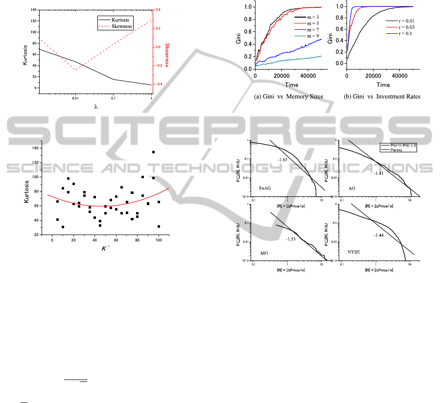
tails. In other words, the more the patterns of price

ﬂuctuation occur, the smaller the kurtosis becomes.

Thus, if λ is small and the reversal movements of con-

trarians are rare, the kurtosis becomes large. On the

other hand, if we vary K

−

with keeping K

= 500,

the kurtosis is distributed as shown in Figure 5, where

a regression curve is depicted.

Figure 4: Skewness and kurtosis vs λ in ExAG.

Figure 5: Kurtosis vs K

−

in ExAG.

From the observation above, we set λ = 0.001,

−

= 50 and K

= 500 in what follows.

For the second issue, we present our results in Fig-

ure 6. The Gini coefﬁcient is used as a measure of

inequality of wealth distribution. Given a set of N

agents’ wealth (X

,. ..,X

), the Gini coefﬁcient G

is deﬁned as

G =

∑

i=1

∑

j=1

− X

where X =

∑

i=1

/N. If G = 0, the wealth is com-

pletely even. If G is close to 1, an agent has a

monopoly on the wealth.

Figure 6(a) shows that the inﬂuence of memory

size on the Gini coefﬁcient. It means that the smaller

the memory size is, the wider the inequality of wealth

becomes. If the memory size is small, some success-

ful agents earn much money and the others not. So

their mean asset values are widely distributed in the

long run. Thus, the Gini coefﬁcient tends to be large.

Figure 6(b) shows that the inﬂuence of invest-

ment rate on the Gini coefﬁcient. It means that the

larger the investment rate is, the wider the inequal-

ity of wealth becomes. If the investment rate is large,

the successful agents earn much money and the others

not. So their mean asset values are widely distributed

in the long run. Thus, the Gini coefﬁcient tends to be

large.

Figure 6: Inﬂuence on Gini coefﬁcient in AG.

Figure 7: Pareto indices for several games and NYSE.

For the third issue, Figure 7 shows the price de-

creasing change distribution for several games and

NYSE, where NYSE is the Dow-Jones industrial av-

erage 20,545 data (1928 /10/1 — 2010/7/26) in New

York Stock Exchange. That is, the normalized de-

creasing change of price |R| = |∆Price/σ| and its dis-

tribution is compared. The straight lines represent the

Pareto indices. At a glance, the curves of ExAG and

AG resemble that of NYSE, which means their dis-

tributions are likewise. The Pareto index of ExAG is

also not far from that of NYSE.

For the fourth issue, we obtained the following re-

sults. Both ExAG and AG have better values of skew-

ness and kurtosis than MG does as shown in Tables 2

and 3, where “stdev.” and “95% int.” mean standard

deviation and 95% conﬁdence interval, respectively.

For the ﬁfth issue, we present our results in Figure

8. The volatility is deﬁned as the standard deviation

of the number of excess demand. The ﬁgure shows

that the volatility of AG is lower than other games for

ICAART 2012 - International Conference on Agents and Artificial Intelligence

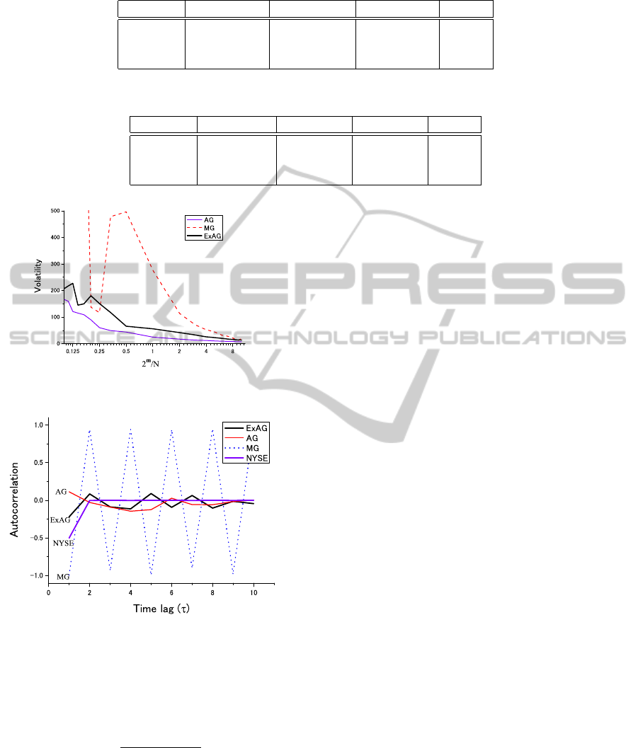
Table 2: Skewness.

method ExAG AG MG NYSE

average 0.098 0.39 -0.32 3.725

stdev. 1.82 1.03 1.86 —

95% int. [-0.58,0.77] [0.007,0.77] [-1.02,0.37] —

Table 3: Kurtosis.

method ExAG AG MG NYSE

average 42.3 72.9 148 18.92

stdev. 61.6 96.3 231 —

95% int. [21.3,67.3] [36.9,109] [62.2,235] —

Figure 8: Volatility (N = 51 ∼ 5119, S = 4, m = 9).

Figure 9: Autocorrelation of volatility.

every memory size. This means the memory size does

not have a great impact on the price formation in AG.

For the sixth issue, the autocorrelation function

C(τ) is deﬁned as

C(τ) =

hA(t)A(t + τ)i

hA(t)

where τ is a time lag. The value of C(τ) becomes 1

(respectively, -1) if there is a positive (respectively,

negative) correlation between A(t) and A(t + τ). As

shown in Figure 9, only MG has the alternating,

strong positive/negativecorrelation for every time lag.

Other games, AG and ExAG, have weak correlations

which reduce as the time lag grows. The practical

data, NYSE, has a negative correlation only when the

time lag is τ = 1. Since the excess demand in NYSE

is unknown, we assume the number of agents is equal

to N = 501 and estimate A(t) from the equation (7).

Notice that ExAG has the same (negative) correlation

as NYSE when τ = 1, while AG has the positive cor-

relation.

5 CONCLUSIONS

In this paper, we proposed an asset value game and

an extended asset value game. The AG is a simple

variant of MG such that the only difference is their

payoff functions. Though the AG captures a good

feature of an agent’s behavior, there is a time lag be-

tween the rapid change of a price and the adjustment

of an agent’s behavior. So we consider the ExAG, an

improvement of AG, by using parameters which con-

tain some probabilistic behavior. The ExAG has two

parameters by which the balance of trend-followers

and contrarians can be controlled. We examined sev-

eral values for the parameters and then ﬁxed to speci-

ﬁed values. We obtained several experimental results

which reveals some characteristics of ExAG. The ad-

vantages of ExAG are twofold. First, we can restrict a

drastic movement of price in AG by tuning the param-

eters. Second, we can reduce the time lag generated

by recovering score losses in AG.

Our future work includes investigating the inﬂu-

ence of market intervention, an in-depth analysis of

the AG, and other applications of the games.

ACKNOWLEDGEMENTS

This work was partially supported by Grant-in-Aid

for Scientiﬁc Research (C) 22510147 of the Ministry

of Education, Science, Sports and Culture of Japan.

A NEW VARIANT OF THE MINORITY GAME - Asset Value Game and Its Extension

REFERENCES

Andersen, J. V. and Sornette, D. (2003). The $-game. The

European Physical Journal B, 31(1):141–145.

Araujo, R. M. and Lamb, L.C. (2004). Towards understand-

ing the role of learning models in the dynamics of the

minority game. In Proceedings of the 16th IEEE In-

ternational Conference on Tools with Artiﬁcial Intel-

ligence (ICTAI 2004), pages 727–731.

Araujo, R. M. and Lamb, L. C. (2009). On the use of mem-

ory and resources in minority games. ACM Transac-

tions on Autonomous and Adaptive Systems, 4(2).

Challet, D. (2008). Inter-pattern speculation: beyond mi-

nority, majority and $-games. Journal of Economic

Dynamics and Control, 32(1):85–100.

Challet, D., Marsili, M., and Zhang, Y. C. (2001). Stylized

facts of ﬁnancial markets and market crashes in mi-

nority games. Physica A: Statistical Mechanics and

its Applications, 294(3-4):514–524.

Challet, D., Marsili, M., and Zhang, Y. C. (2005). Minor-

ity games — interacting agents in ﬁnancial markets.

Oxford University Press, New York, ﬁrst edition.

Coolen, A. C. (2005). The mathematical theory of minor-

ity games. Oxford University Press, New York, ﬁrst

edition.

Ferreira, F. F. and Marsili, M. (2005). Real payoffs and

virtual trading in agent based market models. Physica

A: Statistical Mechanics and its Applications, 345(3-

4):657–675.

Ferreira, F. F., Oliveira, V. M., Crepaldi, A. F., and Campos,

P. R. (2005). Agent-based model with heterogeneous

fundamental prices. Physica A: Statistical Mechanics

and its Applications, 357(3-4):534–542.

Giardina, I., Bouchaud, J. P., and Me´zard, M. (2001). Mi-

croscopic models for long ranged volatility correla-

tions. Physica A: Statistical Mechanics and its Ap-

plications, 299(1-2):28–39.

Kiniwa, J., Koide, T., and Sandoh, H. (2009). Analysis of

price behavior in lazy $-game. Physica A: Statistical

Mechanics and its Applications, 388(18):3879–3891.

Liu, X., Liang, X., and Tang, B. (2004). Minority game and

anomalies in ﬁnancial markets. Physica A: Statistical

Mechanics and its Applications, 333:343–352.

Marsili, M. (2001). Market mechanism and expectations in

minority and majority games. Physica A: Statistical

Mechanics and its Applications, 299(1-2):93–103.

Martino, A. D., Giardina, I., and Mosetti, G. (2003). Statis-

tical mechanics of the mixed majority-minority game

with random external information. Journal of Physics

A: Mathematical and General, 36(34):8935–8954.

Takayasu, H., Miura, T., Hirabayashi, T., and Hamada, K.

(1992). Statistical properties of deterministic thresh-

old elements — the case of market price. Physica

A: Statistical Mechanics and its Applications, 184(1-

2):127–134.

Yamada, K., Takayasu, H., and Takayasu, M. (2007). Char-

acterization of foreign exchange market using the

threshold-dealer-model. Physica A: Statistical Me-

chanics and its Applications, 382(1):340–346.

ICAART 2012 - International Conference on Agents and Artificial Intelligence