STRATEGIC DOMINANCE AND DYNAMIC PROGRAMMING FOR
MULTI-AGENT PLANNING
Application to the Multi-Robot Box-pushing Problem
Mohamed Amine Hamila
1
, Emmanuelle Grislin-Le Strugeon
1
, Rene Mandiau
1
and
Abdel-Illah Mouaddib
2
1
LAMIH, Universite de Valenciennes, Valenciennes, France
2
GREYC, Universite de Caen Basse-Normandie, Caen, France
Keywords:
Multi-agent planning, Coordination, Stochastic games, Markov processes.
Abstract:
This paper presents a planning approach for a multi-agent coordination problem in a dynamic environment. We
introduce the algorithm SGInfiniteVI, allowing to apply some theories related to the engineering of multi-agent
systems and designed to solve stochastic games. In order to limit the decision complexity and so decreasing
the used resources (memory and processor-time), our approach relies on reducing the number of joint-action
at each step decision. A scenario of multi-robot Box-pushing is used as a platform to evaluate and validate our
approach. We show that only weakly dominated actions can improve the resolution process, despite a slight
deterioration of the solution quality due to information loss.
1 INTRODUCTION
Many daily situations involve a decision making: for
example an air-traffic controller has to assign landing-
area and time slots to planes, or a taxi company that
has some transportation tasks to be carried out. Intel-
ligent agents can aid in this decision-making process.
In this paper, we address the problem of collision-free
paths for multiple agents sharing and moving in the
same environment.
The objective of this work is to propose an effi-
cient answer to such coordination problems. One an-
swer is to consider stochastic games, since they pro-
vide a powerful framework for modeling multi-agent
interactions. Stochastic games were first studied as
an extension of matrix games (Neumann and Morgen-
stern, 1944) to multiple states. They are also seen as
a generalization of Markov decision process (MDP)
(Puterman, 2005) to several agents. The Nash equi-
librium (Nash, 1950) is the most commonly-used so-
lution concept, intuitively defined as a particular be-
havior for all agents, where each agent acts optimally
with regard to the others’ behavior.
This work aims to improve the performance of a
previous algorithm, the SGInfiniteVI (Hamila et al.,
2010), designed to solve stochastic games. The latter
allowed finding a decentralized policy actions, based
on the dynamic programming technique and Nash
equilibria. However, the computed solution is made
through a comprehensive process, thereby limiting
the dimensions of the addressed problem.
Our contribution is mainly threefold; firstly, we
present an exact algorithm for the elimination of
weakly/strictly dominated strategies. Secondly, we
have incorporated this technique into the algorithm
SGInfiniteVI, in order to simplify the decision prob-
lems and accelerate the resolution process. Thirdly,
we propose an experimental approach for the evalua-
tion of the resulting new algorithm and it is performed
in two stages; (1) numerical evaluation: attempts to
compare the effect of the elimination of weakly and
strictly dominated strategies, on the used resources,
(2) Behavioral evaluation: checks the impact of the
chosen strategy on the solution quality.
The paper has been organized as follows. Section
2 recalls some definitions of stochastic games. Sec-
tion 3 describes the algorithm SGInfiniteVI, the pro-
cess improvement and shows how to apply on a grid-
world game. Results are presented and discussed in
section 4 and finally we conclude in section 5.
2 BACKGROUND
In this section, we present on one hand an introduc-
91
Amine Hamila M., Grislin-Le Strugeon E., Mandiau R. and Mouaddib A..
STRATEGIC DOMINANCE AND DYNAMIC PROGRAMMING FOR MULTI-AGENT PLANNING - Application to the Multi-Robot Box-pushing Problem.
DOI: 10.5220/0003707500910097
In Proceedings of the 4th International Conference on Agents and Artificial Intelligence (ICAART-2012), pages 91-97
ISBN: 978-989-8425-96-6
Copyright
c
 2012 SCITEPRESS (Science and Technology Publications, Lda.)

tion to the model of stochastic games and on the other
hand some of its crucial aspects.
2.1 Definitions and Concepts
Stochastic Games (SG) (Shoham et al., 2003; Hansen
et al., 2004) are defined by the tuple:
< Ag,{A
i
: i = 1.. .|Ag|},{R
i
: i = 1.. .|Ag|},S,T >
• Ag: is the finite set of agents.
• A
i
: is the finite set of actions (or pure strategies)
available to agent i (i ∈ Ag).
• R
i
: is the immediate reward function of agent i,
R
i
(a) → R, where a is the joint-action defined as
a ∈ ×
i∈Ag
A
i
and is given by a = ha
1
,.. .,a
|Ag|
i.
• S: is the finite set of environment states.
• T: is the stochastic transition function,
T : S × A × S → [0, 1], indicating the probability
of moving from a state s ∈ S to a state s
0
∈ S by
running the joint-action a.
The particularity of stochastic games is that each
state s can be considered as a matrix game M(s). At
each step of the game, the agents observe their envi-
ronment, simultaneously choose actions and receive
rewards. The environment transitions stochastically
into a different state M(s
0
) with a probability P(s
0
|s,a)
and the above process repeats. The goal for each
agent is to maximize the expected sum of rewards it
receives during the game.
2.2 Equilibrium in Stochastic Games
Stochastic games have reward functions which can
be different for every agent. In certain cases, it may
be difficult to find policies that maximize the perfor-
mance criteria for all agents. So in stochastic games,
an equilibrium is always looked for every state. This
equilibrium is a situation in which no agent, taking the
other agents’ actions as given, can improve its perfor-
mance criteria by choosing an alternative action: we
find here the definition of the Nash equilibrium (Nash,
1950).
Definition 1. A Nash Equilibrium is a set of strate-
gies (actions) a
∗
such that:
R
i
(a
∗
i
,a
∗
−i
) > R
i
(a
i
,a
∗
−i
) ∀i ∈ Ag, ∀a
i
∈ A
i
(1)
2.2.1 Strategic Dominance
When the number of agents is large, it becomes dif-
ficult for everyone to consider the entire joint-action
space. This may involve a high cost of matrices con-
struction and resolution. To reduce the joint-action
set, most research (in the game theory) focused on
studying the concepts of plausible solutions. Strate-
gic dominance (Fudenberg and Tirole, 1991; Leyton-
Brown and Shoham, 2008) represents one of the most
widely used concept, seeking to eliminate actions that
are dominated by others actions.
Definition 2. A strategy a
i
∈ A
i
is said to be strictly
dominated if there is another strategy a
0
i
∈ A
i
such as:
R
i
(a
0
i
,a
−i
) > R
i
(a
i
,a
−i
) ∀a
−i
∈ A
−i
(2)
Thus a strictly dominated strategy for a player
yields a lower expected payoff than at least one other
strategy available to the player, regardless of the
strategies chosen by everyone else. Obviously, a ra-
tional player will never use a strictly dominated strat-
egy. The process can be repeated until strategies are
no longer eliminated in this manner. This prediction
process on actions, is called ”Iterative Elimination of
Strictly Dominated Strategies” (IESDS).
Definition 3. For every player i, if there is only one
solution resulting from the IESDS process, then the
game is said to be dominance solvable and the solu-
tion is a Nash equilibrium.
However, in many cases, the process ends with a large
number of remaining strategies. To further reduce
the joint-action space, we could relax the principle of
dominance and so include weakly dominated strate-
gies.
Definition 4. A strategy a
i
∈ A
i
is said to be weakly
dominated if there is another strategy a
0
i
∈ A
i
such as:
R
i
(a
0
i
,a
−i
) > R
i
(a
i
,a
−i
) ∀a
−i
∈ A
−i
(3)
Thus the elimination process would provide more
compact matrices and consequently reduce the com-
putation time of the equilibrium. However, this pro-
cedure has two major drawbacks: (1) the elimination
order may change the final outcome of the game and
(2) eliminating weakly dominated strategies, can ex-
clude some Nash equilibria present in the game.
2.2.2 Best-response Function
As explained above, the iterative elimination of dom-
inated strategies is a relevant solution, but unreliable
for an exact search of equilibrium. Indeed discarding
dominated strategies narrows the search for a solu-
tion strategy, but does not identify a unique solution.
To select a specific strategy requires to introduce the
concept of Best-Response.
Definition 5. Given the other players’ actions a
−i
,
the Best-Response (BR) of the player i is:
BR
i
: a
−i
→ argmax
a
i
∈A
i
R
i
(a
i
,a
−i
) (4)
ICAART 2012 - International Conference on Agents and Artificial Intelligence
92

Thus, the notion of Nash equilibrium can be ex-
pressed using the concept of Best-Response:
∀i ∈ Ag a
∗
i
∈ BR
i
(a
∗
−i
)
2.3 Solving Stochastic Games
The main works on planning in stochastic games
are the ones of Shapley (Shapley, 1953) and Kearns
(Kearns et al., 2000). Shapley was the first to pro-
pose an algorithm for stochastic games with an in-
finite horizon for the case of zero-sum games. The
FINITEVI algorithm by Kearns et al., generalizes the
Shapley’s work to general-sum case.
In the same area, the algorithm SGInfiniteVI
(Hamila et al., 2010) brought several improvements,
including the decentralization and the implementation
of the equilibrium selection function (previously re-
garded as an oracle), in the aim to deal with complex
situations, such as the equilibrium multiplicity.
However, the algorithm reaches its limits as the
problem size increases. Our objective consists in im-
proving the algorithm SGInfiniteVI by eliminating
useless strategies, with the aim to accelerate the com-
putation time, to reduce the memory usage and to plan
easily with fewer coordination problems.
3 INTEGRATION OF THE
DOMINANCE PROCEDURE
AND APPLICATION
In this section we present the dominance procedure
(IEDS) and how we integrate it into the SGInfiniteVI
algorithm.
3.1 The Improvement of SGInfiniteVI
We first present the algorithm 1, which performs the
iterative elimination of dominated strategies (intro-
duced in Section 2). The algorithm takes as parameter
a matrix M(s) of an arbitrary dimension and returns a
matrix M
0
(s) assumed to be smaller. The elimination
process is applied iteratively until each player has one
remaining strategy, or several strategies none of which
being weakly dominated. Note that each player will
seek to reduce its matrix, not only by eliminating its
dominated strategies but also those of the others.
The IEDS is incorporated into the algorithm (Al-
gorithm 2, line 8) in the aim to:
• Significantly reduce the matrix size: if after the
procedure, there is more than one strategy per
player (line 12), the equilibrium selection must be
refined to favor a strategy over another one. Thus,
Best-Response function is used to find equilibria.
• Directly calculate a Nash equilibrium: this hap-
pens when the intersection of all strategies (one
per player) forms a Nash equilibrium (line 8).
Algorithm 1: IEDS algorithm.
Input: a matrix M(s)
1 for k ∈ 1...|Ag| do
2 for stratCandidate ∈ A
k
do
3 stratDominated ← true
4 for stratAlternat ∈ A
k
do
5 if stratCandidate non-dominated by
stratAlternat then
6 stratDominated ← false
7 if stratDominated then
8 delete stratCandidate from A
k
Output: |M
0
| ≤ |M|
Algorithm 2: The SGInfiniteVI algorithm with
IEDS.
Input: A stochastic game SG, γ ∈ [0,1], ε ≥ 0
1 t ← 0
2 repeat
3 t ← t + 1
4 for s ∈ S do
5 for a ∈ A do
6 for k ∈ 1...|Ag| do
7 M(s,a,k,t) = R
k
(s,a) +
γ
∑
s
0
∈S
T (s, a,s
0
) V
f
k
(M(s
0
,a,t −1))
8 M’(s,t) = IEDS (M(s,t))
9 if |M
0
| = 1 then
10 π
k
(s,t) = f
join
(M
0
(s,t))
11 else
12 π
k
(s,t) = f (M
0
(s,t))
f



f
NashMaxTot
maximizes the payoffs of agents.
f
NashMaxSub
maximizes its own payoff.
f
ApproxNash
selects an approximate Nash.
13 until max
s∈S
|V
f
(s,t) −V
f
(s,t −1)| < ε;
Output: Policy π
i
Note that in case of equilibrium multiplicity, we
propose two selection functions
1
: one function maxi-
mizes the overall gain f
NashMaxTot
and the other max-
imizes the individual gain f
NashMaxSub
. If there is no
equilibrium then we use the function f
ApproxNash
to
reach an approximate Nash equilibrium.
1
We propose only the functions f
NashMaxTot
and
f
NashMaxSub
because it has been shown that these functions
were better than the NashPareto in case of equilibrium mul-
tiplicity.
STRATEGIC DOMINANCE AND DYNAMIC PROGRAMMING FOR MULTI-AGENT PLANNING - Application to
the Multi-Robot Box-pushing Problem
93

Algorithmic Complexity. In the search for equi-
libria, the algorithm is dealing only with a pure
Nash equilibrium. It has been proved that whether a
game has a “pure Nash equilibrium” is NP-complete
(Conitzer and Sandholm, 2008). Therefore, the run-
ning time of SGInfiniteVI algorithm is not polynomial
in the size of the game matrix (due to the fact that the
function f used to compute Nash equilibrium is it-
self non-polynomial). Moreover, the size of the states
space is exponential in the number of agents. The run-
ning time of our algorithm is taken to be exponential.
Spatial Complexity. Since the agent can only keep
the equilibrium values, the total number of required
values is: |S| × |Ag|. SGInfiniteVI is linear in the
number of states and agents
2
. The matrix is com-
posed of |Ag| values, making a total of |Ag| × |A| val-
ues. Every agent can store a backup matrix after each
evaluation of the state s, including its own payoff but
also the payoffs of the other agents. But it is not
necessary, since the agent can only keep the values
of the payments coming from the calculated equilib-
rium. Therefore the total number of required values
is: |S| × |Ag|. SGInfiniteVI is linear in the number of
states and agents
3
.
3.2 Grid-world Game
The example that we choose is similar to the exam-
ples from literature, as the “Two-Player Coordina-
tion Problem” of Hu and Wellman (Hu and Wellman,
2003). It is the problem of multi-robot box-pushing
(see Figure 1), the game includes robots, objects and
a container box. In this example, the objective of the
robots is to put all the objects in the box with a mini-
mum number of steps without conflict.
Figure 1: An example of scenario: two robots, four objects
and a container box.
The following section intends to validate the im-
proved algorithm on the modeled game.
2
the next section will show that this complexity is a
worst-case complexity and that in practice a gain in memory
can be considered.
3
the next section will show that this complexity is a
worst-case complexity and that in practice a gain in memory
can be considered.
4 VALIDATION
The experiments were performed on 200 policies (one
for each agent), with 20, 000 tests per policy (chang-
ing at each test randomly the agents initial position).
The simulator was implemented in Java language and
the experiments were performed on a machine quad-
core 2.8GHz and 4GB of memory.
First, experiments were made to study the effect
of IEDS procedure on the used resources. Second, we
sought to determine its effect on the agents’ behavior.
4.1 Numerical Evaluation
This section aims to demonstrate empirically the ef-
fect of IEDS on the equilibrium computation, the
CPU-time and the memory space (depending on the
type of eliminated strategies).
4.1.1 Equilibrium Computation
We wanted to test the algorithm with two different
procedures (IESDS and IEWDS), respectively per-
forming iterative elimination of strictly and weakly
dominated strategies. The purpose is to know which
of the two procedures would make a profit without
degrading the quality of the solution. The optimal
case of reduction corresponds to one strategy per
player (the joint-action forms an equilibrium). We
call pcRed the percentage of the reduction.
The experiments show that for the case of strictly
dominated strategies, the percentage of Nash equilib-
rium found by the f
join
function is generally less than
20%. As for the elimination of weakly dominated
strategies, the percentage is close to 90% as shown
in Figure 2. The results reflect the ascendancy of the
weakly dominated strategies in terms of matrix reduc-
tion.
0
0.2
0.4
0.6
0.8
1
4 5 6 7 8 9 10 11 12 13 14 15 16
Percentage of Nash equilibria found with IEDS
Grid size
I.E. weakly D.S.
I.E. strictly D.S.
Figure 2: Comparison between IEWDS and IESDS in terms
of matrix reduction (with 2 agents, 4 objects and different
grid size).
ICAART 2012 - International Conference on Agents and Artificial Intelligence
94

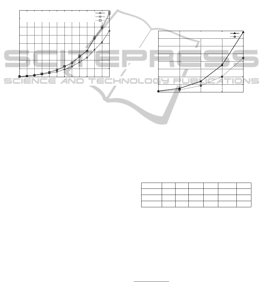
4.1.2 Evaluation on the Computation Time
We compared the computation time used by the al-
gorithm SGInfiniteVI with/without IEDS. The figure
3 shows that the elimination of weakly dominated
strategies provides a significant gain in time G
t
, de-
pending on the size of the environment. Neverthe-
less, the use of strictly dominated strategies does not
reduce the computation time but increases it a little.
Outside the context of the application, we can say that
0
50
100
150
200
250
300
350
400
4 5 6 7 8 9 10 11 12 13 14 15 16
Time in seconds
Grid size
Elimination of weakly dominated strategies
Without IEDS
Elimination of strictly dominated strategies
Figure 3: Comparison between IEWDS, IESDS and the
original version of the algorithm, in terms of computation
time (with 2 agents, 4 objects and different grid size).
the reduction of the matrix size is not necessarily syn-
onymous of less computation time. Indeed, the IEDS
procedure leads to a gain g
t
on the exploration time of
the matrix, but also entails a computational cost c
t
in
addition to the one of the algorithm, the useful gain is
being given by the difference g
t
− c
t
.
Thus, to obtain a gain in time G
t
that is percepti-
ble at the general level, the degree of reduction pcRed
must be large enough to generate a gain g
t
covering
c
t
. The parameter pcRed could be integrated into the
algorithm to allow launching (if required) the IEDS
procedure.
4.1.3 Evaluation on Memory Space
At this level, the used dominance procedure does not
allow to reduce directly the memory usage, but pro-
pose an estimation of the gain. Indeed, a gain is pos-
sible only when matrices are partially calculated. For
example, it is useless to calculate the payments of the
other players, when these coincide with a dominated
and therefore not performed strategy. An estimate of
the expected gain can be made from the average num-
ber of dominated strategies per player. The scenario
is the following one:
1. Each player computes only its own payments. The
number of calculated values is: |A|,
2. Start the IEDS process,
3. Calculate the payments of the other players when
they only correspond to the surviving strategies.
The number of new values filled in the matrix is:
|A
−i
|, which makes a total of |A|+|A
−i
| by matrix,
4. Find the best-response,
The expected gain per matrix is then:
g
m
= (nbrValMat − nbrValCalc) / nbrValMat
= ( (|A| ∗ |Ag|) − (|A| +|A
−i
|) ) / (|A| ∗|Ag|)
The total expected gain is:
G
m
= g
m
∗ pcRed
= ( (|A| ∗ |Ag|) − (|A| +|A
−i
|) ) ∗ pcRed
0
200
400
600
800
1000
1200
1400
1600
4 5 6 7 8
Used memory space (MB)
Grid size
Used memory without IEDS
Used memory with IEDS
Figure 4: Memory space required to calculate a policy (with
3 agents, 3 objects and different grid size).
The table 1 shows the evolution of the expected
gain according to the number of agents and the figure
5 shows in practice the evolution of the expected gain
according to the problem size. The empirical analysis
of g
m
and pcRed leads to an estimated gain G
m
of
about 40%.
Table 1: Expected gain according to the number of agents.
|A
g
| |A| |M| g
m
pcRed G
m
2 agents 2 25 50 40% ' 90% 35%
3 agents 3 125 375 60% ' 75% 45%
4 agents 4 625 2500 70% ' 53% 37%
This will allow considering higher problem sizes,
increasing the number of agents, the grid size, etc.
4.2 Evaluation on the Agents’ Behavior
To assess the effect of the elimination of dominated
strategies
4
on the agents’ behavior; we define three
elements of comparison:
4
We consider only weakly dominated strategies, since
the elimination of strictly dominated strategies cannot make
significant gains.
STRATEGIC DOMINANCE AND DYNAMIC PROGRAMMING FOR MULTI-AGENT PLANNING - Application to
the Multi-Robot Box-pushing Problem
95

• The average number of conflicts: a conflict is con-
sidered when agents violate any of the game rules,
e.g. an agent moving to a position that is already
occupied by another agent.
• The average number of deadlocks: a deadlock oc-
curs when agents are preventing each other’s ac-
tions forever, waiting for a shared resource.
• The average number of livelocks: a livelock is an
endless cycle that prevents the agents from reach-
ing a goal state, and the game from any progress.
4.2.1 Average Number of Conflicts
Figure 5 shows that the elimination of dominated
strategies leads to an increase in the number of con-
flicts compared to the original version of the algo-
rithm. Nevertheless, the observed values remain rela-
tively small and can be considered as acceptable in the
context of the simulation. For example, for a simula-
tion with a grid size of 12 × 12, two agents and four
objects, the average number of conflicts is only 0.25
per simulation.
0
0.05
0.1
0.15
0.2
0.25
0.3
4 6 8 10 12 14 16
The average number of conflicts/simulation
Grid size
Without IEDS
With IEDS
Figure 5: Evaluation according to the average number of
conflicts (with 2 agents, 4 objects and different grid size).
4.2.2 Average Number of Deadlocks and
Livelocks
The figure 6 shows a slight increase in the average
number of deadlocks by simulation compared to the
original version of the algorithm. The number of
deadlocks may reflect a loss in terms of coordination
between agents. Indeed, such a situation occurs when
the actions performed from distinct Nash equilibria.
4.2.3 Conclusion of the Experimentation
We found that results show a significant gain in com-
putation time and an opportunity to gain memory
space. Intuitively, this gain is not without conse-
quence on the agents’ policies. Dominated strategies
0.35
0.4
0.45
0.5
0.55
0.6
0.65
4 6 8 10 12 14 16
The average number of deadlocks/simulation
Grid size
Without IEDS
With IEDS
Figure 6: Evaluation according to the average number of
deadlocks (with 2 agents, 4 objects and different grid size).
may affect long-term gains, even though they are con-
sidered unnecessary during the elimination process.
In addition, adopting the concept of dominance sim-
plifies the decision problem at each stage by getting
rid of the equilibrium multiplicity.
5 CONCLUSIONS
In the context of coordinating agents, the aim of this
work was not only to study the model of stochastic
games, but also to propose a planning algorithm based
on the dynamic programming and the Nash equilib-
rium. Our method involves the implementation, the
validation and the evaluation on an example of in-
teraction between agents. The concept of strategic
dominance has been studied and used in order to im-
prove the SGInfiniteVI algorithm computation time
and used memory. The experiments demonstrated
that only the elimination of weakly dominated strate-
gies could make a gain in time and memory.
REFERENCES
Conitzer, V. and Sandholm, T. (2008). New complexity re-
sults about nash equilibria. Games and Economic Be-
havior, 63(2):621–641.
Fudenberg, D. and Tirole, J. (1991). Game theory. MIT
Press, Cambridge, MA.
Hamila, M. A., Grislin-le Strugeon, E., Mandiau, R., and
Mouaddib, A.-I. (2010). An algorithm for multi-robot
planning: Sginfinitevi. In Proceedings of the 2010
IEEE/WIC/ACM International Conference on Web In-
telligence and Intelligent Agent Technology - Volume
02, WI-IAT ’10, pages 141–148, Washington, DC,
USA. IEEE Computer Society.
Hansen, E. A., Bernstein, D. S., and Zilberstein, S.
(2004). Dynamic programming for partially observ-
able stochastic games. In Proceedings of the 19th na-
ICAART 2012 - International Conference on Agents and Artificial Intelligence
96

tional conference on Artifical intelligence, AAAI’04,
pages 709–715. AAAI Press.
Hu, J. and Wellman, M. (2003). Nash q–learning for
general–sum stochastic games. Journal of Machine
Learning Research, 4:1039–1069.
Kearns, M., Mansour, Y., and Singh, S. (2000). Fast plan-
ning in stochastic games. In In Proc. UAI-2000, pages
309–316. Morgan Kaufmann.
Leyton-Brown, K. and Shoham, Y. (2008). Essentials of
game theory: A concise multidisciplinary introduc-
tion. Synthesis Lectures on Artificial Intelligence and
Machine Learning, 2(1):1–88.
Nash, J. F. (1950). Equilibrium points in n-person games.
Proc. of the National Academy of Sciences of the
United States of America, 36(1):48–49.
Neumann, J. V. and Morgenstern, O. (1944). Theory of
games and economic behavior. Princeton University
Press, Princeton. Second edition in 1947, third in
1954.
Puterman, M. (2005). Markov Decision Processes: Dis-
crete Stochastic Dynamic Programming. Wiley-
Interscience.
Shapley, L. (1953). Stochastic games. Proc. of the National
Academy of Sciences USA, pages 1095–1100.
Shoham, Y., Powers, R., and Grenager, T. (2003). Multi-
agent reinforcement learning: a critical survey. Tech-
nical report, Stanford University.
STRATEGIC DOMINANCE AND DYNAMIC PROGRAMMING FOR MULTI-AGENT PLANNING - Application to
the Multi-Robot Box-pushing Problem
97