ENGINE CALIBRATION PROCESS OPTIMIZATION
Erica Klampfl, Jenny Lee, David Dronzkowski and Kacie Theisen
Ford Research & Advanced Engineering, 2101 Village Road, Dearborn, MI, U.S.A.
Keywords:
Set-covering, Binary integer programming, Engine calibration.
Abstract:
Before an engine can be scheduled in the Product Development cycle for inclusion in a vehicle, it must be
calibrated in such a way that it satisfies a variety of regulatory tests over a range of conditions. The current
engine calibration process involves conducting a design of experiments at a representative number of steady
state points in order to satisfy all required regulatory tests: test engineers use a standard 16 × 16 grid with
standard grid spacing and then conduct a design of experiments on a subset of those points - about 120 of
them. This work explores how to reduce the engine calibration process time by finding the best 16× 16 grid
choice (i.e. the best spacing on both the engine speed and torque axes) and the minimum number of points
on the grid to test in order to satisfy regulatory constraints around NO
X
, particulate matter, noise, and fuel
consumption. Our proposed method models the problem as a Binary Integer Program that simultaneously
selects the best grid spacing and optimized number of points to test, while guaranteeing that all specified
constraints hold. We present an example that demonstrates how we can reduce the number of necessary test
points by approximately 56%.
1 INTRODUCTION
As vehicle emission and fuel economy standards con-
tinue to tighten, manufacturers respond by develop-
ing increasingly more complex engine systems with
advanced control strategies. The process of calibrat-
ing such an engine (i.e. assigning the desired val-
ues to control parameters) quickly becomes a daunt-
ing task for calibration engineers. In the case of a
modern internal combustion engine that may have
six or more inputs (e.g. injection timings, injec-
tion quantities, intake manifold pressure, and ex-
haust gas recirculation rate), generating data for the
calibration task is a time consuming and costly en-
deavor. If we consider the simple case where the re-
sponse of the engine could be reasonably modeled
with a quadratic function (i.e. each control factor
can be understood by using three settings), and the
engine speed and load regime (i.e. the range of en-
gine rotational speed and available output torque) are
each segmented by 16 grid quadrants, then the cal-
ibration engineer would be need to run 16
2
× 6
3
=
256×4,096= 55,296 test points: this is derived from
the (number of quadrants)
engine speed×torque
× (number
of inputs)
number of settings
. At roughly 5 minutes per
test point, data collection alone would take over six
months! Confound this with the fact that calibrations
must be developed for different operating conditions
and engine operation modes, and the product devel-
opment timeline quickly becomes uncompetitive.
There has been significant work using design
of experiment (DoE) and mathematical optimization
techniques to minimize the amount of input data
needed for every given speed and load combina-
tion (e.g. (Yoshida et al., 2011), (Maloney, 2009),
(Castagn´e et al., 2008), and (Langou¨et et al., 2008)):
the goal is to reduce the number of inputcombinations
to some fraction of the possible combination of in-
puts and settings (e.g. 6
3
= 4, 096 combinations when
there are six inputs and three settings). However, this
work does not address on which of the 16
2
= 256
speed and load combinations (i.e. test points) a cali-
bration engineer should focus their efforts, as it is not
feasible to consider every combination. This selection
of test points needs to be determined in such a way to
satisfy testing of typical transient drive cycles needed
to pass certification (i.e. the Environmental Protec-
tion Agency (EPA) Federal Test Procedure (FTP) 75
test cycle (EPA, 1977)).
Steady state (SS) engine development consists of
maintaining constant speed and load for prolonged
periods of time (e.g. five minutes or more). This is
not, however, typical of how most vehicle owners op-
erate their vehicles. Vehicles are usually driven in
335
Klampfl E., Lee J., Dronzkowski D. and Theisen K..
ENGINE CALIBRATION PROCESS OPTIMIZATION.
DOI: 10.5220/0003695603350341
In Proceedings of the 1st International Conference on Operations Research and Enterprise Systems (ICORES-2012), pages 335-341
ISBN: 978-989-8425-97-3
Copyright
c
 2012 SCITEPRESS (Science and Technology Publications, Lda.)

a transient manner with engine speed and load con-
stantly changing with pedal position. The transient
test in Figure 1 is a discretized version of an FTP test,
but note that the time spent at any of these points is
less than one second.
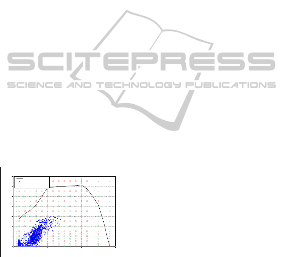
Figure 1 illustrates a conventional 16 × 16 grid
(calibration table points), a discretized representation
of a transient drive cycle (FTP74 Test Points), typi-
cal engine calibration test points, and an engine’s full
load curve (FLC). The transient drive cycle, usually
mandated by a regulatory agency such as the EPA,
is intended to represent a “typical” vehicle’s driving
pattern. The engine calibration test points are usually
a subset of the 256 possible speed and load combina-
tions discussed above. The FLC essentially represents
the output capability of the engine. The typical engine
test points denoted by circles in Figure 1 include all
points directly above and below the FLC, all points on
the zero axis, and every other grid point. The current
process involves performing some level of calibration
work: in-vehicle idle validation for zero load points
for idle and off-idle performance, set point mapping
at the FLC to ensure hardware limits are maintained,
and a DoE at selected points to ensure emissions com-
pliance and minimize fuel consumption. The work
included in this paper is an attempt to minimize the
number of speed/load points to test and to find the
best grid location for these points instead of always
considering a fixed subset of points as demonstrated
by the calibration test points in Figure 1. The goal
is to expedite the product development life-cycle and
significantly reduce testing costs.
400 800 1200 1600 2000 2400 2800 3200 3600 4000
Engine Speed [RPM]
Torque [Nm]
0
200
400
600
800
1000
1200
1400
Full Load Curve
FTP74 Test Points
Calibration Table Points
Calibration Test Points
Figure 1: Typical engine operating regime.
2 PROBLEM FORMULATION
We model this problem as an Binary Integer Pro-
gram (BIP), where all functions are linear, and all
decision variables are binary. This problem is re-
lated to set-covering problems (Balas and Padberg,
1972), (Wolsey, 1998), where we find the minimum-
cost cover. However, in the traditional set covering
problems, the points from which to determine the
cover are pre-defined. In our problem, we have to
simultaneously determine both the points from which
to select the cover (i.e. which SS points will be in the
grid) and the best cover (i.e. which SS points we will
test). We consider that a transient point or SS point
not selected in the grid is covered by a selected SS
point if it is within a certain distance to any selected
SS point.
2.1 Inputs
The inputs below describe the necessary information
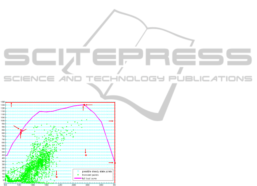
to run the model: several are illustrated in Figure 2.
E
s
= engine speed starting point = min
k
{FLE
k
}.
E
e
= engine speed ending point = max
k
{FLE
k
}.
T
s
= torque starting point.
T
e
= torque ending point = max
k
{FLTU
k
}.
p = length/width dimensions of final grid.
GX
min
= minimum allowed for the grid to be spaced
in the engine speed direction.
GY
min
= minimum allowed for the grid to be spaced
in the torque direction.
q = number of possible grid points on x-axis
r = number of possible grid points on y-axis
n = q×r number of possible SS points.
m = number of transient points.
K = {1,.. . ,q} : set of grid point indices on x-axis.
R = {1,.. . ,r} : set of grid point indices on y-axis.
S = {1,.. . ,n} : set of possible SS points.
I = {1,.. . ,m} : set of transient points.
dt
ij
= distance between transient point i ∈ I and
possible SS point j ∈ S.
ds
j
1
j
2
= distance between two SS points j
1
, j
2
∈ S.
DT
max
= max distance allowed between a transient
point and its closest selected SS point.
DS
max
= max distance allowed between a SS point
and its closest selected SS point.
DX
max
= max grid spacing in x direction.
DY
max
= max grid spacing in y direction.
E
j
= engine speed j ∈ S.
T
j
= torque j ∈ S.
FE
max
= max engine speed value of FLC.
FT
max
= max torque value of FLC.
FLE
k
= FLC engine speed value ∀ k ∈ K.
FLT
k
= FLC torque value ∀ k ∈ K.
FLTU
k
= FLC torque upper value ∀ k ∈ K.
FLTD
k
= FLC torque lower value ∀ k ∈ K.
We define the m× n incidence matrix A and n× n
incidence matrix B as follows
a
ij
=

1 if dt
ij
≤ DT
max
0 otherwise
∀ i ∈ I and j ∈ S
ICORES 2012 - 1st International Conference on Operations Research and Enterprise Systems
336

b
j
1
j
2
=

1 if ds
j
1
j
2
≤ DS
max
0 otherwise
∀ i, j ∈ S
Figure 2 is illustrative of many of the input pa-
rameters. It shows the FLC on the grid of all pos-
sible SS points, which are denoted by circles. The
transient points are superimposed on this figure and
are denoted by stars. The torque value, T
e
= 1300
TRQ, corresponds to the SS point that is directly
above the highest point on the FLC. In this figure,
FT
max
= 1255 TRQ is just slightly above the pos-
sible SS point, x
1897
, which has a torque value of
1250; hence, T
e
is giventhe next highest torque value,
1300 TRQ. There are a total of n = 1755 possible SS
points. In our implementation, the indexing scheme
for each possible SS point starts from the bottom left
corner of the grid and continues up from left to right
(see Figure 3). Each possible SS point has an asso-
ciated engine speed and torque, but is not indexed
over engine speed and torque. For example, in Fig-
ure 2 x
161
is a SS point with an engine speed, E
161
,
and a torque, T
161
, where (E
161
,T
161
) = (2100,100).
Also shown in the Figure are FE
max
= 3800 RPM,
E
e
= 3800 RPM, (FLE
10
,FLT
10
) = (1050,818.25),
FLTD
10
= 800 TRQ, and FLTU
10
= 850 TRQ.
Engine Speed (RPM)
Torque (TRQ)
T
e
FLTU
10
(FLE
10
,FLT
10
)
FLTU
10
(E
161
, T
161
)
(E
161
, T
161
)
x
1897
FT
max
FE
max
E
e
Figure 2: This figure shows all possible grid points in the
engine speed and torque space labeled with example input
parameters.
2.2 Variables
In this section, we introduce the decision variables for
the model. The first binary variable will determine if a
possible SS point will be included in the 16× 16 grid.
x
j
=



1 if j ∈ S is selected to be a SS
point in the 16× 16 grid
0 otherwise
The second binary variable will determine which
of the SS points that are selected to be included in the
16× 16 grid will have a DoE run at that point. These
selected points will have to cover the other grid points
for which a DoE will not be run and cover all transient
points:
y
j
=



1 if j ∈ S is a SS point selected for
testing
0 otherwise
2.3 Objective Function
Our objective function is currently to minimize the
size of the cover. Since we consider all points in the
cover of equal value, we are just minimizing the num-
ber of SS points needed to cover the transient points
and all other possible SS points. Our current objective
is to minimize the cover points, which is reflected in
min
∑
j∈S
y
j
. (1)
The objective function could easily account for
different costs associated with each selected point to
include things such as the actual distance between the
cover of SS points and the points it is covering. This
would capture the case where the greater the distance
between the point in the cover and the points it is cov-
ering, the worse the cover. For example, this could
accommodate if the error rate for interpolating a SS
value was worse for a greater distance between the
interpolated point and its cover point. However, this
could increase the number of tested points.
2.4 Constraints
This section describes the cover constraints, as well as
additional constraints that capture certain points that
must be included in the cover, grid spacing require-
ments, and constraints to ensure the resulting grid is
16 × 16. To illustrate these constraints, we introduce
a small example, where p = 6, E
s
= 500, E
e
= 1200,
T
s
= 0, T
e
= 450, GX
min
= 50, GY
min
= 50, DX
max
=
150, and DY
max
= 150. There are q = 12 possible
engine speeds from which to choose for the grid in
the x-direction and r = 10 possible torque values from
which to choose for the grid in the y direction. Note
that in this example we need to choose a 6 × 6 grid
(i.e. 36 points) from a total of 120 points, whereas in
the typical problem we need to choose 256 points to
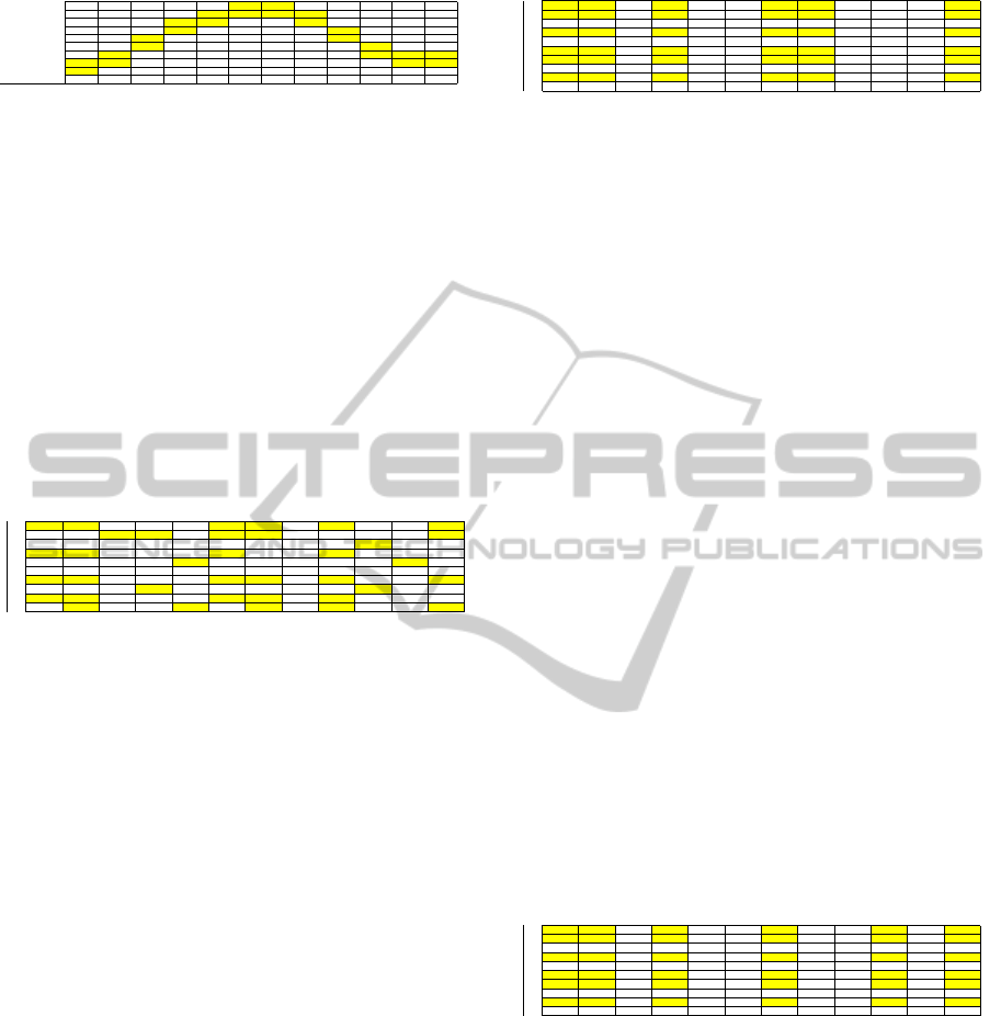
form the grid from a total of 1755 points. Figure 3
shows the indexing scheme for this size problem: the
highlighted indices are the grid points directly above
and below the FLC (i.e. FLTU
k
and FLTD
k
∀ k ∈ K).
ENGINE CALIBRATION PROCESS OPTIMIZATION
337

R Torque
10 450 109 110 111 112 113 114 115 116 117 118 119 120
9 400 97 98 99 100 101 102 103 104 105 106 107 108
8 350 85 86 87 88 89 90 91 92 93 94 95 96
7 300 73 74 75 76 77 78 79 80 81 82 83 84
6 250 61 62 63 64 65 66 67 68 69 70 71 72
5 200 49 50 51 52 53 54 55 56 57 58 59 60
4 150 37 38 39 40 41 42 43 44 45 46 47 48
3 100 25 26 27 28 29 30 31 32 33 34 35 36
2 50 13 14 15 16 17 18 19 20 21 22 23 24
1 0 1 2 3 4 5 6 7 8 9 10 11 12
500 650 700 800 850 900 950 1000 1050 1100 1150 1200
1 2 3 4 5 6 7 8 9 10 11 12
Eng ine Sp eed
K
Figure 3: This figure shows all possible grid points and cor-
responding index from which a 6× 6 grid must be chosen.
2.4.1 Choosing a Grid
The first constraint guarantees that we have exactly
p× p SS points in the grid:
∑
j∈S
x
j
= p× p (2)
Note that this constraint does not guarantee that all
of the points are chosen to be in the same rows and
columns. Figure 4 shows an example selection of 6×
6 = 36 highlighted points that were chosen based on
this constraint, but they do not form a 6× 6 grid.
10 450 109 110 111 112 113 114 115 116 117 118 119 120
9 400 97 98 99 100 101 102 103 104 105 106 107 108
8 350 85 86 87 88 89 90 91 92 93 94 95 96
7 300 73 74 75 76 77 78 79 80 81 82 83 84
6 250 61 62 63 64 65 66 67 68 69 70 71 72
5 200 49 50 51 52 53 54 55 56 57 58 59 60
4 150 37 38 39 40 41 42 43 44 45 46 47 48
3 100 25 26 27 28 29 30 31 32 33 34 35 36
2 50 13 14 15 16 17 18 19 20 21 22 23 24
1 0 1 2 3 4 5 6 7 8 9 10 11 12
0 500 650 700 800 850 900 950 1000 1050 1100 1150 1200
Figure 4: This figure shows highlighted in blue the 6× 6 =
36 points that were chosen to satisfy constraint (2).
The next two constraints address this problem and
guarantee that we have exactly p columns and p rows
chosen to compose the grid. Note that the two con-
straints (3) and (4) make constraint (2) redundant, but
having it improvesthe solve time by around 5% based
on our testing, as it gives a better representation of the
convex hull (typically, additional constraints in BIPs
help improve solve time (Geoffrion, 1976)). The con-
straint to ensure we choose exactly p columns is
∑
j
2
∈S:E
j
1
=E
j
2
x
j
2
= px
j
1
∀ j
1
∈ K. (3)
The following guarantees we choose exactly p rows:
∑
j
2
∈S:T
j
1
=T
j
2
x
j
2
= px
j
1
∀ k ∈ {0,. .. ,r − 1} (4)
∀ j
1
∈ S : j
1
= qk+ 1.
Figure 5 shows an example grid selection, choosing
columns 1, 2, 4, 7, 8, and 12 and rows 2, 4, 5, 7, 9, and
10. The next few constraints enforce maximum spac-
ing between the grid points in both the engine speed
and torque directions. We ensure that the first (i.e.,
left-most) column in the grid must be at most DX
max
away from the starting value of E
s
:
∑
j∈S:E
j
≤E
1
+DX
max
x
j
≥ p. (5)
10 450 109 110 111 112 113 114 115 116 117 118 119 120
9 400 97 98 99 100 101 102 103 104 105 106 107 108
8 350 85 86 87 88 89 90 91 92 93 94 95 96
7 300 73 74 75 76 77 78 79 80 81 82 83 84
6 250 61 62 63 64 65 66 67 68 69 70 71 72
5 200 49 50 51 52 53 54 55 56 57 58 59 60
4 150 37 38 39 40 41 42 43 44 45 46 47 48
3 100 25 26 27 28 29 30 31 32 33 34 35 36
2 50 13 14 15 16 17 18 19 20 21 22 23 24
1 0 1 2 3 4 5 6 7 8 9 10 11 12
0 500 650 700 800 850 900 950 1000 1050 1100 1150 1200
Figure 5: This figure an example grid with exactly 6 rows
and 6 columns.
Note that in Figure 5, column 1 is selected, and since
E
s
= 500, this constraint holds.
Next, we require the grid to be spaced at most
DY
max
in the torque direction:
x
j
1
+
∑
j
2
∈S:j
2
> j
1
∧|T
j
1
−T
j
2
|≤DY
max
x
j
2
≥ p+
∑
c∈S:T
c
=T
j
1
x
c
(6)
∀ k ∈ {0,. ..,((T
end
− DY
max
)/GY
min
)}
∀ j
1
∈ S : j
1
= qk+ 1.
Following Figure 5, we can see that the maxi-
mum space between any two rows is 100, and since
DY
max
= 100, this constraint holds.
Finally, we guarantee that the grid can be spaced
at most DX
max
in the engine speed direction:
x
j
1
+
∑
j
2
∈S:j
2
> j
1
∧|E
j
1
−E
j
2
|≤DX
max
x
j
2
≥ p+
∑
c∈S:E
c
=E
j
1
x
c
(7)
∀ j
1
∈ {1,.. .,((E
end
− DX
max
− E
s
)/GX
min
+ 1)}.
Following Figure 5, we can see that the maximum
space between any two columns is 200 (e.g. columns
8 and 12), and since DX
max
= 150, this constraint is
violated. Figure 6 shows a grid selection that satisfies
all constraints up to this point, with a maximum space
between any two columns equal to 150.
10 450 109 110 111 112 113 114 115 116 117 118 119 120
9 400 97 98 99 100 101 102 103 104 105 106 107 108
8 350 85 86 87 88 89 90 91 92 93 94 95 96
7 300 73 74 75 76 77 78 79 80 81 82 83 84
6 250 61 62 63 64 65 66 67 68 69 70 71 72
5 200 49 50 51 52 53 54 55 56 57 58 59 60
4 150 37 38 39 40 41 42 43 44 45 46 47 48
3 100 25 26 27 28 29 30 31 32 33 34 35 36
2 50 13 14 15 16 17 18 19 20 21 22 23 24
1 0 1 2 3 4 5 6 7 8 9 10 11 12
0 500 650 700 800 850 900 950 1000 1050 1100 1150 1200
Figure 6: This figure is an example grid selection that satis-
fies all constraints in Section 2.4.1.
2.4.2 Required Grid Points
There are a couple of types of SS points that are re-
quired to be a part of the grid. The first require-
ment forces the grid to contain points that have values
greater than or equal to the max torque on the FLC.
This is equivalent to forcing the maximum value in
the grid to be selected.
∑
j∈S:T
j
=T
e
x
j
= p. (8)
ICORES 2012 - 1st International Conference on Operations Research and Enterprise Systems
338

Similarly, the grid has to contain points that have val-
ues greater than or equal to the max engine speed on
the FLC.
∑
j∈S:E
j
=E
e
x
j
= p. (9)
We can see that the grid of chosen SS points in Figure
6 satisfies these two constraints because row 10 and
column 12 are selected.
The next requirement is that points on the zero
axis must be selected:
∑
j∈K
x
j
= p. (10)
Note that the grid of chosen SS points in Figure 6
does not satisfy this constraint because row 1 is not
selected. Figure 7 shows a grid selection that satis-
fies this constraint, as well as all of the constraints
in Section 2.4.1. Note that selected rows have been
changed: row 1 instead of row 2 and row 3 instead of
row 4 to maintain DY
max
= 100.
10 450 109 110 111 112 113 114 115 116 117 118 119 120
9 400 97 98 99
100 101 102 103 104 105 106 107 108
8 350 85 86 87 88 89 90 91 92 93 94 95 96
7 300 73 74 75
76 77 78 79 80 81 82 83 84
6 250 61 62 63 64 65 66 67 68 69 70 71 72
5 200 49
50 51 52 53 54 55 56 57 58 59 60
4 150 37 38 39 40 41 42 43
44 45 46 47 48
3 100
25 26 27 28 29 30 31 32 33 34 35 36
2 50 13 14 15 16 17 18 19 20 21 22 23 24
1 0
1 2 3 4 5 6 7 8 9 10 11 12
0 500 650 700 800 850 900 950 1000 1050 1100 1150 1200
Figure 7: This figure is an example grid selection that sat-
isfies constraints (2) - (15) with the cells containing the
indices above and below the FLC outlined and the cover
points in large, bold text.
2.4.3 Cover Constraints
This section describes the standard cover constraints
and also additional constraints needed to require cer-
tain selected grid points to be in the cover. The first
standard type of cover constraints guarantee that all
transient points are covered:
∑
j∈S
a
ij
y
j
≥ 1 ∀ i ∈ I. (11)
Next, we ensure that all SS points that are not in the
cover are covered:
∑
j
2
∈S
b
j
1
j
2
y
j
2
≥ 1 ∀ k ∈ K : E
k
≤ E
end
∀ j
1
∈ S : (12)
T
j
1
≤ FLTU
k
∧ E
j
1
= FLE
k
.
The following constraints are not standard cover-
ing constraints: they guarantee that the points directly
above and below the FLC are not only included in the
selected grid but are also selected as part of the cover.
First, though, we must ensure that if a point is chosen
to be part of the cover, then it must have been selected
to be a part of the grid:
y
j
≤ x
j
∀ j ∈ S. (13)
Next, we guarantee that p SS points directly above the
FLC are selected to test:
∑
k∈K:E
k
≤E
end
∑
j∈S:T
j
=FLTU
k
∧E
j
=FLE
k
y
j
= p. (14)
Additionally, we guarantee that p SS points directly
below the FLC are selected to be in the cover:
∑
k∈K:E
k
≤E
end
∑
j∈S:T
j
=FLTD
k
∧E
j
=FLE
k
y
j
= p. (15)
Finally, we must ensure that all the SS points in the
selected grid that are above the point directly chosen
above the FLC are not selected as a part of the cover:
∑
k∈K
∑
j∈S:T
j
>FLTU
k
∧E
j
=FLE
k
y
j
= 0. (16)
Figure 7 shows an example selected grid that sat-
isfies all of the constraints: the indices in the high-
lighted cells represent the selected grid, the indices di-
rectly above and below the FLC are outlined in black,
and the cover points are denoted by large, bold text.
We used IBM ILOG CPLEX Optimization Studio
12.2 (IBM, 2010) to solve the BIP. CPLEX takes on
average 90 minutes to obtain an optimal solution.
3 EXAMPLE
The following example is of the grid and SS test point
selection for a typical internal combustion engine.
The target of this model application is to reduce the
number of speed/load point combinations necessary
to develop an engine calibration that delivers equiva-
lent performance in terms of NO
X
, particulate, noise,
and fuel consumption.
3.1 Inputs
We provide the values for the inputs introduced in
Section 2.1. Refer to Figure 2 for a pictorial of the
entire grid space, the FLC, and the transient points
for the internal combustion engine in this example.
In Table 1, we provide the values for the engine
start and end speed, the torque start and end speed,
the grid dimensions, minimum grid spacing in the
engine and torque grid directions, maximum engine
speed and torque for the FLC, and cover require-
ments. Other parameters that are calculated from
these values are the number of possible grid points
ENGINE CALIBRATION PROCESS OPTIMIZATION
339

along the x-axis, the y-axis, and the number of possi-
ble SS points: q =
E
e
−E
s
+GX
min
GX
min
=
3800−600+50
50
= 65,
r =
T
e
−T
s
+GY
min
GY
min
=
1300−0+50
50
= 27, and n = q × r =
65× 27 = 1755.
Table 1: Input Parameters: scalar numbers.
Param. Value Unit Param. Value Unit
E
s
600 RPM n 1755
E
e
3800 RPM m 2618
T
s
0 TRQ DT
max
300
T
e
1300 TRQ DS
max
300
p 16 DX
max
550 RPM
GX
min
50 RPM DY
max
150 TRQ
GY
min
50 TRQ FE
max
3800 RPM
q 65 FT
max
1255 TRQ
r 27
We define the sets for the engine speed and torque
grid point indices, the possible SS points, and the
transient points as follows: K = {1,. .. ,65}, R =
{1,...,27}, S = {1, .. ., 1755}, and I = {1,...,2618}.
The engine speed, E
j
, starts with 600 RPM and ends
at 3800 RPM with an increment of 50 RPM. Torque,
T
j
, has a starting point of 0 TRQ and increments by
50 TRQ with a maximum of 1300 TRQ. The dis-
tance between possible SS point j
1
and j
2
for ev-
ery j
1
, j
2
∈ S is calculated using the Euclidean For-
mula d =
p
(x
2
− x
1
)
2
+ (y
2
− y
1
)
2
, where x
1
and x
2
are the engine speed of j
1
and j
2
, and y
1
and y
2
are
the corresponding torque values. Similarly, we use
the Euclidean distance formula to calculate the dis-
tance between all transient points i ∈ I and SS points
j ∈ S. As there are 2,619 transient points, we do
not include them in this paper. The following points
on the FLC are in terms of engine speed (RPM) and
torque (TRQ): (0,373), (650, 445), (800, 623), (1000,
778), (1200, 939), (1400, 1061), (1600, 1147), (1800,
1140), (2000, 1152), (2200, 1185), (2400, 1205),
(2600, 1234), (2900, 1255), (3000, 1209), (3200,
1117), (3400, 979), and (3800, 325).
3.2 Results
In this section, we present the optimization grid spac-
ing and test point results for the internal combustion
engine used in our study. We will also demonstrate
how the selected grid and test points satisfy all con-
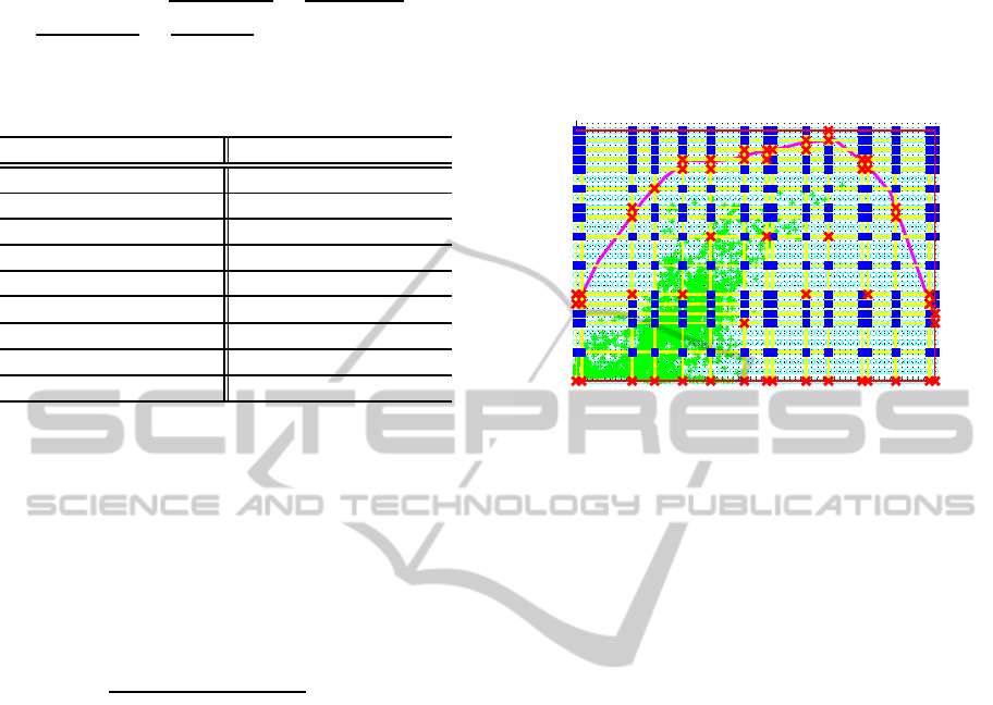
straints.
First, we can see in Figure 8, the selected grid
points (defined by the 256 selected SS points) for
the 16 × 16 grid. This grid selection satisfies the
constraints specified in (2), (3), and (4) to have ex-
actly 256 points chosen, with exactly 16 rows and 16
columns. In addition, the maximum spacing between
the grid points in this example in the engine speed
direction is 550 RPM and 150 TRQ in the torque di-
rection, which satisfies constraints (5), (6), and (7).
600 1000 1400 1800 2200 2600 3000 3400 3800
0
50
100
150
200
250
300
350
400
450
500
550
600
650
700
750
800
850
900
950
1000
1050
1100
1150
1200
1250
1300
Egine Speed (RPM)
Torque (TRQ)
Figure 8: 54 Selected SS Points.
Furthermore, we confirm that the selected grid
points satisfy i) constraints (8) and (9) that require the
grid to contain points that have values greater than or
equal to the max engine speed and max torque on the
FLC; and ii) constraint (10) that forces the points on
the zero axis to be selected. Figure 8 shows three lines
that represent these grid constraints and demonstrate
that our solution satisfies them.
The second part of our solution identifies which
of the grid points are selected as SS points to test.
Our solution yields a minimum number of 54 out of
256 SS points to test, which are identified by an X
in Figure 8. We can see that test points are selected
only from points that have been chosen to be in the
grid: this satisfies constraint (13). Also note that all
16 SS points directly above and below the FLC are
selected to be tested, and none of the points beyond
the 16 points above the SS points are chosen to be
tested: this satisfies constraints (14), (15), and (16).
Finally, we demonstrate how all of the transient
points and SS points that were not selected for testing
are covered by the SS points selected for testing (con-
straints (11) and (12)). Figure 9 shows which points
are covered by the selected test points. Each selected
test point, denoted by an X, has a radius of 300 that
is marked by a circle. Any transient point or SS point
that is in the circle is covered by that SS point at the
center of the circle: note that due to different scaling
in the torque and engine axes, the circles appear as
ellipses. We can see that all of the transient and SS
points that were not selected for testing are covered
by at least one of the 54 SS points selected for testing.
For this example, the current testing process for
the internal combustion engine would have required
ICORES 2012 - 1st International Conference on Operations Research and Enterprise Systems
340

600 1000 1400 1800 2200 2600 3000 3400 3800
0
50
100
150
200
250
300
350
400
450
500
550
600
650
700
750
800
850
900
950
1000
1050
1100
1150
1200
1250
1300
Engine Speed (RPM)
Torque (TRQ)
Figure 9: This figure shows the coverage of non-selected
transient and SS points.
testing 122 points with the standard grid spacing. Our
method selects a different grid spacing and chooses
only 54 points to test, giving us around a 56% reduc-
tion in the number of points needed for testing.
4 SUMMARY
Completing a DoE at all possible steady-state engine
operating points is a time consuming process. This
project focused not on reducing the time to complete
the DoE, but on reducing the number of experiments
that needed to be performed. We captured the con-
straints to ensure that by minimizing the number of
tests to perform, we could still satisfy regulatory re-
quirements and internal testing constraints.
We introduced a BIP formulation that is based on
a set-covering approach to select the best grid dimen-
sions and to minimize the number of SS points. This
formulation yields an optimal solution to simultane-
ously solving the grid selection and covering prob-
lem. We demonstrated the optimization methodology
for a typical internal combustion engine and provided
an optimal grid selection that resulted in an approxi-
mately 56% reduction in the points for which to per-
form a DoE.
While we applied this approach to the area of en-
gine calibration, this method could also be applied to
other automotive related areas. One example would
be to select the minimum number of points on a sur-
face on which to weld in order to satisfy certain ma-
terial properties. Another example would be to min-
imize the number of stamping facilities and to deter-
mine the best locations to add stamping facilities in
order to guarantee that every assembly plant would
have at least one stamping facility within a certain
distance. These are just a couple of examples that
illustrate the diverse types of problems for which this
approach can be applied.
REFERENCES
Balas, E. and Padberg, M. (1972). On the set coverying
problem. Operations Research, 20:1152–1161.
Castagn´e, M., Bentolila, Y., Chaudoye, F., Hall´e, A., Nico-
las, F., and Sinoquet, D. (2008). Comparison of engine
calibration methods based on design of experiments
(DoE). Oil & Gas Science and Technology, 63:563–
582.
EPA (1977). Title 40 - protection of environment, CFR § 86
subpart B.
Geoffrion, A. (1976). A guided tour of recent practical
advances in integer linear programming. OMEGA,
The international Journal of Management Science,
4(1):49–57.
IBM (2010). IBM ILOG CPLEX opti-
mization studio (OPL). http://www-
01.ibm.com/software/integration/optimization/cplex-
optimization-studio/.
Langou¨et, H., M´etivier, L., Sinoquet, D., and Tran, Q.
(2008). Optimization for engine calibration. In En-
gOpt 2008 - International Conference on Engineering
Optimization. Rio de Janeiro, Brazil.
Maloney, P. (2009). Objective determination of minimum
engine mapping requirements for optimal SI DIVCP
engine calibration. Warrendale: SAE International.
Wolsey, L. (1998). Integer Programming. John Wiley &
Sons, Inc.
Yoshida, S., Ehara, M., and Koroda, Y. (2011). Rapid
boundary detection for model-based diesel engine cal-
ibration. Warrendale: SAE International.
ENGINE CALIBRATION PROCESS OPTIMIZATION
341