DEVELOPING COMBINED FORECASTING MODELS

IN OIL INDUSTRY

A Case Study in Opec Oil Demand

Seyed Hamid Khodadad Hosseini

, Adel Azar

, ALi Rajabzadeh Ghatari

and Arash Bahrammirzaee

Department of Management, Tarbiat Modares University (TMU), Tehran, Iran

Iran Management and Productivity Center Researcher, Tehran, Iran

Keywords: Energy forecasting, Neural network forecasting, Combined forecasting, Oil demand.

Abstract: The purpose of this research is to study the combined forecasting methods in energy section. This method is

a new approach which leads to considerable reduction of error in forecasting results. In this study,

forecasting has been done through using individual methods (these methods consist of exponential

smoothing methods, trend analysis, box-Jenkins, causal analysis, and neural network models) and also

combining methods. In next step, the Results of these individual forecasting methods have been combined

and compared with artificial neural networks, and multiple regression models. The data we used in this

study are: dependent variable: OPEC oil demands from 1960 to 2005, and independent variables: oil price,

GDP, other energy demands, population, and added-value in industry (in OECD countries. Computed

indexes of errors are: MSE, MAPE, and GAPE which show considerable reductions in the errors of

forecasting when using combining models. Therefore, it is suggested that the designed models could be

applied for oil demand forecasting.

1 INTRODUCTION

Decision making about energy and other related

problems in our chaotic world is a crucial issue for

managers at national level, and also for large,

middle, and small enterprises. Any changes in

energy consumption rate considerably influence

related decisions and plans. Due to numerous

variables in this area, managers and experts prefer to

have some mechanisms to help them make

appropriate decisions. Forecasting OPEC

(Organization of Petroleum Exporting Countries)

crude oil demand is a relatively difficult task which

represents two essential attributes: on the one hand,

it shows the strong daily changes and on the other, it

clearly shows the increasing trend. Mostly, the

prediction of oil industry is based on time series

analysis. Time series methods are affected by other

variations that make the problem hard to model.

Some of the researchers aimed to propose models

which consider affective factors on crude oil

(Medlock and Ronald, 1999). Factors, such as the

rate of population change, industrial growth or

decline, the added value of industry, government

regulations, and energy-thrift policies have been

identified as effective items on energy demand

changes (Schrattenholzer, 2004). Therefore, a

complex model, taking into account the effects of

these individual parameters, might seem to be

necessary when predicting energy-demand changes

(Mackay and Probert, 2001).

The conventional time series modeling methods

have served the scientific community for a long

time; however, they provide only reasonable

accuracy and suffer from the assumptions of

stationary and linearity. Among the traditional

model, one of the most important and widely used

time series models is the autoregressive integrated

moving average (ARIMA). The popularity of the

ARIMA model is due to its statistical properties as

well as the well-known Box–Jenkins methodology

(Box and Pierce, 1970).

Among new methods, Artificial Neural Networks

(ANNs) are considered as efficient tools for

modeling and forecasting during the last two

decades. The major advantage of neural networks is

their flexible nonlinear modeling capability. With

ANNs, there is no need to specify a particular model

form. Rather, the model is adaptively formed based

205

Khodadad Hosseini S., Azar A., Rajabzadeh Ghatari A. and Bahrammirzaee A..

DEVELOPING COMBINED FORECASTING MODELS IN OIL INDUSTRY - A Case Study in Opec Oil Demand.

DOI: 10.5220/0003681702050210

In Proceedings of the International Conference on Neural Computation Theory and Applications (NCTA-2011), pages 205-210

ISBN: 978-989-8425-84-3

 2011 SCITEPRESS (Science and Technology Publications, Lda.)

on the features presented from the data (Zhang et al.,

2001).

However, there are extensive researches in

forecasting domain, especially in financial domain

(Bahrammirzaee, 2010), but a few researches have

been conducted on oil demand predictions using

intelligent techniques (e.g., Assareh et al., 2010).

This shortage makes much more sense in a country

like Iran with huge oil consumption, and therefore

demands. This issue is central focus point of this

article. In the next section, the process of selection

of variable, sample, and data gathering will be

detailed.

This paper is organized as follows: first, based

on previous researches and also documented OPEC

crude oil studies, the affected variables are selected.

The prediction has been done separately by classic

methods and ANN algorithm, and then the combined

methods is suggested for such a prediction.

2 VARIABLES, SAMPLE AND

DATA GATHERING

Most of the oil market studies are based on classic

forecasting methods. For example, in 2007,

(Dochuchaev, 2007) have done a research on

effective factors in oil and demand price by studying

structure’s evolution and price revolutions. The

research of (Petrov et al., 2004), introduce some

effective factors such as political factors.

The variables which have been extracted based

on extensive review of researches (Oil Market

Report, 1993-2005); (OPEC Annual Bulletin, 2000);

(OPEC Oil and Energy Data, 1980-2005); (Arab Oil

and Gas Directory,1985-2005). are as follows:

1. Crude oil price.

2. Income of the countries which are consumers of

OPEC oil, namely members of OECD. (GDP and

economic growth).

3. The population level and the population growth

rate of OECD countries.

4. Other kinds of energy consumption, e.g. gas,

electrical energy, nuclear energy.

5. The Added-Value of the industrial sector of

OECD countries.

As cited before, these variables have been selected

based on the literature review which has been done

by authors, but because of the limited related studies

in this area, we tried to extend these factors by

taking expert’s opinions acquisition. For formulating

variables, designing check lists using Delphi

methods is done. Delphi method is used for

minimizing deviation among the experts. After

determining these variables, the related data sets

consisting of OPEC oil demand rates from 1960 to

2005, as dependent variable and price, GDP,

population, added- value in industry and other

demands for energy, as independent variables are

obtained. Data acquired from 1960 to 1996 were

used as sample data, and from 1997-2005 as testing

data.

Methods used in this research for forecasting are

quantitative methods. These methods include time-

series analysis (mono-variable analysis including

exponential smoothing, trends analysis, Box-

Jenkins) and causal analysis (econometric, ANN).

These methods which are called individual methods

are used for predicting oil demand, and then these

methods are combined. The combination is done by

neural network, multiple regression, and sequential

methods.

3 MODELING AND DATA

ANALYSIS

The following separated steps are done for modeling

the crude oil demand prediction:

Step 1: Forecasting Oil Demand using Classic

Methods: We used classic methods and their

analyses as follows:

1. Exponential Smoothing Forecasting Methods:

This method includes some separated forecasting

such as:

Simple Brown: This is a forecasting method using

an adjustment coefficient which reduces forecasting

errors. After analyzing this data driven method, the

smoothing coefficient was equal to 0.1 (α= 0.1).

This amount is computed by trial and error and takes

the best result for the sum of the square of errors.

Holt Smoothing Method: This method also predicts

through an adjustment coefficient which reduces

forecasting errors. After analyzing this method, the

smoothing coefficient was equal to 0.7 (α= 0.1) and

β (trend coefficient) equal to 0.4.

This amount is computed by trial and error which

takes the minimum amount of the sum of the square

of errors.

Custom Smoothing with Linear Trend: Similar to

the Holt method, α= 0.7 and β= 0.45 are the most

proposed coefficients.

Custom Smoothing with Exponential Trend:

Forecasting results have shown the best amount of

NCTA 2011 - International Conference on Neural Computation Theory and Applications

206

their error with α= 0.7 and β= 0.45 in this method.

Like other smoothing methods, parameters are

computed by trial and error.

Custom Smoothing with Damped Trend:

Forecasting by Damped trend is done using three

parameters: α,β and δ. The smoothing coefficients

are equal to α= 0.1,β= 0.1 and δ= 0.1. By using

these parameters the sum of square of the errors are

at a minimum.

The detailed results of errors are illustrated in

Table 5.

2. Forecasting by using Trend Analysis Method:

Different trends are analyzed in trend analysis as

follow: 1.Linear Trend, 2.Logarithmic Trend,

3.Inverse Trend, 4.Quadratic Trend, 5.Cubic trend,

6.Power Trend, 7.Compound Trend, 8.S- curve

Trend, 9.Logistic Trend, 10.Growth Trend,

11.Exponential Trend

For finding the best trend, all above trends are

formulated. The best trends are selected by

considering their R2 and MSE. ANOVA (analysis of

variance) results confirm that linear trend,

logarithmic trend, quadratic trend, and compound

trend are the most suitable trends. Equations of

selected trends are listed in Table 1:

Table 1: Most suitable Trend Equations.

The detailed error results are illustrated in Table 5.

3. Forecasting by using Box- jenkins Method: In

Box- Jenkins models (ARIMA), the following

analyses for statistical modeling were carried out:

1. Determination of normality and stationary of data.

2. Using Box-Cox conversion for normalizing data and

using differentiation for stationary data.

3. Computing auto-correlation coefficients, charts, and

studying partial auto-correlation coefficients.

According to this statistical modeling [ARIMA (1, 1,

1)], parameter p equals 1, parameter q equals 1, and

parameter d equals 1. The error results of this model

and their amounts are illustrated in Table 5.

4. Econometrics Causality Methods: In these

models, the behavior of affected data is studied. The

forecasting is done by formulating the dependent

variable using the effects of independent variables.

The variables and abbreviations used in causal

modeling are shown as follow:

= OPEC oil demand during time t.

= Oil price during time t.

GDP= Gross Domestic Product of countries

which are OPEC oil consumers (OECD).

= Demand for other kind-s of energy

during time t.

VAI= Added Value for industrial parts for

countries which are OPEC oil consumers.

The causal models that are obtained are illustrated in

Table 2. This Table shows the equations and also

their analysis.

In the first model, oil demand has a significant

relationship with oil price, GDP and also with other

substitution energies demand (OE). In model (2) the

relationships are logarithmic and independent

variables which have been inputted in the model are

GDP, OE and also VAE. The relationship shows the

price elasticity and also revenue elasticity with oil

demand. Model (3) is a hybrid model consisting

ARIMA and regression model. Like model (3),

model (4) is a hybrid model with combination of

MA (1). Model (5) is a long term oil demand model

with the delay demand which has been inputted in

the model. The demand’s data sets which have been

imported in the model are belonging to previous

year (one year delay). This model (5) is not

considered in combining methods, because of its

correlation within its inputted variables.

In all models p-value<=.05, Determination

coefficient R

and adjusted R

are approximately

equal to 0 .9., Durbin Watson statistics equal to 2,

and all p-values are significant for variables and

constant quantity. The error results of causal

methods are shown in Table 5.

Step 2: Forecasting Oil Demand by Neural

Networking Method: The supervised back

propagation is widely used for time series

forecasting. Therefore we decided to choose this

well-known method for forecasting OPEC oil

demand. Consequently, normalizing data, training

data and weighting the network’s inputs have been

done. Topology is selected based on continuous

changes, especially changes in the amount of the

hidden layer's neurons. The best Neural Network

Model is (5, 15,1) in which internal layer is with 15

neurons, and one output of oil demand is obtained.

Functions of middle layer are considered as sigmoid

function and transfer function is considered as linear

function. The result of errors of Neural Network

Model is shown in Table 5. The topology is similar

to combined ANN model with different numbers of

neurons and the input layers.

Step 3: Combining Individual Forecasting

Method: In this step, combining individual forecas-

DEVELOPING COMBINED FORECASTING MODELS IN OIL INDUSTRY - A Case Study in Opec Oil Demand

207

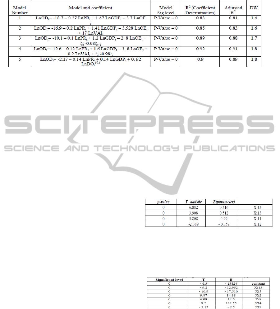
Table 2: The causal equations.

ting methods is done. Individual models which are

used in this combination are as follows:

: Simple Brown Smoothing Methods.

: Holt.

: Custom Exponential Smoothing with 2

parameters.

: Custom Exponential Smoothing with 1

parameter.

: Damped Exponential Smoothing.

: Linear Trend.

: Quadratic Trend.

: Logarithmic Trend.

: Combining Trend.

i10

: ARIMA (1, 1, 1).

i11

: Econometric-s (First Model: independent

variables are price variables, Gross National

Product, and other energies) - Logarithmic Model .

i12

: Econometrics (Second Model:independent

variables are price variables, Gross National

Product, and other energies)- Logarithmic Model

plus Moving Average (MA).

i13

: Econometrics(Third Model).

i14

: Neural Network (MLP with Back Propagation).

Combining individual forecasting models is done by

using following methods:

1. Combining Individual Forecasting Methods

using Artificial Neural Network Models: We have

used supervised Multi-Layer Perceptron (MLP) back

propagation neural network in this research. In this

combination, the results of 14 individual forecasting

models (including 5 exponential smoothing models,

4 trend models, 1 ARIMA model, and 4 casual

methods) are combined. Result of each forecasting

method is considered as an input. By allocating

weights to each input, network topology is

considered with 14 inputs, 30 neurons as hidden

layer and one output layer. Transfer function used is

sigmoid function. In this model Gross Domestic

Product (GDP), oil price, consumption of other

energy resources, population and finally industrial

added- value are used as independent variables.

2. Combining Individual Forecasting Model

using Multi-variable Regression: In this

combination, the results of 14 individual forecasting

models (including 5 exponential smoothing models,

4 trend models, 1 ARIMA model, and 4 casual

methods, 1 neural network model) are combined.

Independent variables xi11, xi12, xi13… xi14 (i= 1,

2… 43) are results of individual forecasting methods

and the dependent variable is actual oil demand data

during research period (i=1,2, …, 43). The fitted

regression model use stepwise method. Fitness of

the model and the parameters are shown in Table 3.

Table 3: Significances of combined model (A).

In addition to this model, other combinations

with regression models are analyzed, and one model

without using neural network is selected. Fitness of

model and its parameters is shown in Table 4.

Table 4: Significances of combined model (B).

3. Combining with Sequential Algorithm:

Combination of smoothing method and ARIMA

method is done with sequential algorithm. The

smoothing methods results with no statistical model

can be combined with the ARIMA model with

statistical modeling. Different results of smoothing

methods have been entered in ARIMA model and

the best model is selected. Five smoothing methods

are entered into ARIMA model and fine combined

NCTA 2011 - International Conference on Neural Computation Theory and Applications

208

models are selected. ARIMA (1, 1, 1) is results of

this combination and the result of errors is shown in

Table 4. In the exponential smoothing method we

don’t have statistical modeling but the advantage of

this combination is that we can have a model.

However, n this way we cannot have considerable

reduction in the errors. This combined model is

working to telecommunication analysis, in which the

output of first model can be considered for input of

the second model.

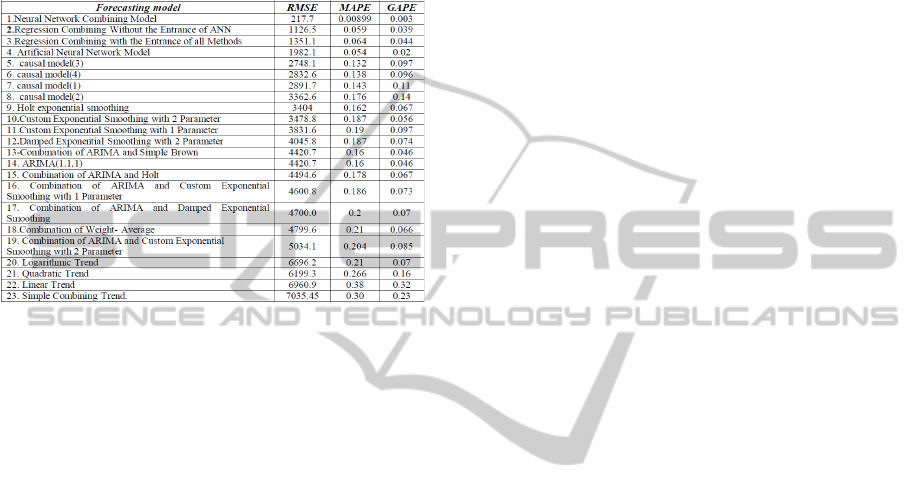
4. Comparison of Forecasting Methods: The

comparison of forecasting methods is done based on

error indexes. In analyzing error indexes,

Armestrong et al. (1992), and Trapson (1990),

indexes been used in this research consisting RMSE,

MAPE, and GAPE.

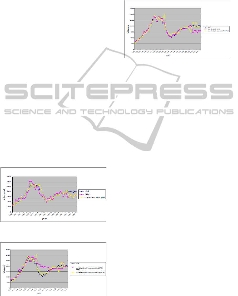
The results of these comparisons are shown in Table

5. The comparisons are done by percentage of the

MSE. In Figures (1), (2), and (3), the comparisons of

three combined methods results, and ANN algorithm

results with real data are shown. This inter-sample

comparisons show the similarity of ANN errors with

combined ANN errors, and two other combining

methods with each other. We also have done t-test

for comparing results and the significant level (p-

value>=.05) which shows that the results doesn’t

have significant mean differences.

In this Figure, the result of combined model with

ANN and real data are compared. As we mentioned

before the mix model is done with ANN algorithm.

Figure 1: Comparison of real data with ANN/combined

ANN results.

Figure 2: Comparison of real data with two kinds of

combined regression results.

In Figure 2, the result of combined model with

regression and ANN, and the combined model with

regression without ANN are compared.

Figure 3: Comparison of real data with combined Model

method results.

As we can see in these Figures, the results of all

combination are very close, and this shows the good

performance of the combining model.

4 CONCLUSIONS AND

RECOMMENDATION

The main derived conclusions could be summarized

as follows:

1. Among different individual methods used in this

study, RMSE of ANN forecasting method provided

better results in oil demand forecasting. Oil demand

data are naturally chaotic, so because of the high

ability of artificial neural network (ANN) method in

training data and allocating suitable weights to this

data, results show the better capability of ANN for

forecasting oil demand comparing to other

individual forecasting methods.

2. Multi-variable Regression Method will do

multiple correlation tests, and therefore it omits

some of the variables in this process. But in ANN

method, all of the inputs (models) could be

considered in forecasting process. Also, based on

previous studies been reviewed in this article, ANN

method can be a useful and effective method for

combining, because in this method combining will

be done on the outputs and each of them can be

considered as absolutely independent inputs. So, if

the objective is to obtain minimum errors for

forecasting, the ANN is suggested. However, it must

be noted that ANN cannot provide the statistical

modeling.

3. Combining Exponential Smoothing with Box-

Jenkins model could not decrease the amounts of

error of each Smoothing method, and Box-Jenkins

DEVELOPING COMBINED FORECASTING MODELS IN OIL INDUSTRY - A Case Study in Opec Oil Demand

209

model separately. Based on RMSE, this combination

has an upper error level than each individual

method. However, for statistical modeling,

combination of exponential Smoothing with ARIMA

can be useful and effective.

Table 5: Models Errors Comparison and Computed Error

Standards (Original Standard is considered MSE).

4. Since in combination theories, weighted average

method is a well-known method, in present study,

this method has been used by applying weighted

based on MSE index.

In this combination analysis, weighted average has

not been like an appropriate combining method, and

its error reduction is not considerable.

The overall results of this research show

justification and feasibility of different combining

models for forecasting oil demand in OPEC, and

other energy resources suppliers. For future works,

an expert system could also be designed which can

be used to select the best method among all

combining methods.

REFERENCES

Arab Oil and Gas Directory,1985-2005.

Armstrong J. S., Collopy F., (1992). Error Measures for

generalizing about forecasting methods: Empirical

Comparison, International Journal of Forecasting 8:

69-80.

Assareh E., Behrang M. A., Assari M. R., Ghanbarzadeh

A (2010). Application of PSO (particle swarm

optimization) and GA (genetic algorithm) techniques

on demand estimation of oil in Iran. 35(12): 5223-

5229.

Bahrammirzaee A., (2010). A Comparative Survey of

Artificial Intelligence Applications in Finance:

Artificial Neural Networks, Expert System and Hybrid

Intelligent Systems, Neural Computing and

Application, 19(8): 1165-1195.

Box, G. E. P. and Pierce D. A., (1970). Distribution of

Residual Autocorrelations in Atuoreressive-Integrated

Moving Average Models. J. American Stat. Assoc. 65:

1509–1526.

Dochuchaev E. S., Rogacheva A. M., Evtushenko E. V.,

(2007). The Forecasting of the World Oil Price by

Swimming up Linear Trend and Periodic Functions;

Oil and Gas Business.

Mackay R. M., Probert S. D., (2001). Forecasting the

United Kingdom’s supplies and demands for fluid

fossil-fuels, Applied Energy 69: 161–189.

Medlock, K. B., Ronald, S. (1999), The Composition and

Growth of Energy Demand in China, China and Long-

Range Asia Energy Security: An Analysis of the

Political, Economic and Technological Factors, James

Baker III Institute for Public Policy, Rice University.

Oil Market Report, 1993-2005.

OPEC Annual Bulletin, 2000.

OPEC Oil and Energy Data, 1980-2005.

Petrov V. V., Artyushkin V. F., (2004). Prices’ Behavior

on the World Oil Market. Moscow: Fazis, P. 192.

Schrattenholzer L., (2004) Designing environmentally

compatible energy strategies: global E3 scenarios

described by IIASA models, presented at China-IEA

seminar on energy modelling and statistics, Beijing

October 20–21.

Trapson, P., (1990). An MSE statistic for comparing

forecast accuracy across series, Int. Journal of

forecasting 6: 219-227.

Zhang, G., Pattuwo, E. B., Hu, M. Y., (2001). A

simulation Study of Artificial Neural Networks for

Nonlinear Time Series Forecasting, Computers &

Operation Research, 28:381-396.

NCTA 2011 - International Conference on Neural Computation Theory and Applications

210