GENE ONTOLOGY BASED SIMULATION FOR FEATURE
SELECTION
Christopher E. Gillies
1
, Mohammad-Reza Siadat
1
, Nilesh V. Patel
1
and George Wilson
2
1
Department of Computer Science, Oakland University, 2200 N. Squirrel Road, Rochester, Michigan 48309, U.S.A.
2
Research Institute, William Beaumont Hospitals, 3601 W. 13 Mile Rd. Royal Oak, Michigan 48073, U.S.A.
Keywords:
Gene ontology, Gene ontology annotation, Gene expression profile classification, Feature selection, Dimen-
sionality reduction and simulation.
Abstract:
Increasing interest among researchers is evidenced for techniques that incorporate prior biological knowledge
into gene expression profile classifiers. Specifically, researchers are interested in learning the impact on classi-
fication when prior knowledge is incorporated into a classifier rather than just using the statistical properties of
the dataset. In this paper, we investigate this impact through simulation. Our simulation relies on an algorithm
that generates gene expression data from Gene Ontology. Experiments comparing two classifiers, one trained
using only statistical properties and one trained with a combination of statistical properties and Gene Ontol-
ogy knowledge, are discussed . Experimental results suggest that incorporating Gene Ontology information
improves classifier performance. In addition, we discuss the relationship of distance between means of the
distributions of the classes and the training sample size on classification accuracy.
1 INTRODUCTION
Gene expression classification is an important area
of research in bioinformatics. In its simplest form,
a two class gene expression classification problem
compares two classes; (1) a control class, and (2)
a diseased class. Gene expression profiles are col-
lected using DNA microarrays which consist of a set
of probes, where each probe, except control probes,
corresponds to a gene. The probes on the DNA mi-
croarray detect the expression levels of the genes ex-
pressed for a biospecimen. Most microarrays contain
thousands of probes. For example, the Affymetrix
1
HU-133A GeneChip detects the expression levels of
22,215 genes (Papachristoudis et al., 2010). Gene ex-
pression profile classification has many similarities to
other pattern recognition activities which can be listed
in four steps: preprocessing, feature selection, train-
ing, and validation. An analyst is presented with a
a training set T ∈ R
m×n
where m is the number of
genes, and n is the number of biospecimens analyzed
using DNA microarrays. A column of T represents
the gene expression profile of a biospecimen, and a
row of T represents the expression levels for a gene
1
Affymetrix: http://www.affymetrix.com, 3420 Central
Expressway Santa Clara, CA 95051
across all biospecimens. The primary goal for this
analyst is to find T
0
∈ R
d×n
where T
0
⊂ T such that
when a classifier C is trained on T
0
, the accuracy of
C is acceptable and C is generalizable. In the pre-
processing step, an analyst must clean T such that
any missing values are estimated and T is also nor-
malized. The next step is feature selection which is
arguably the most important step. Feature selection
not only increases accuracy of a classifier but also
identifies biomarkers
2
(Saeys et al., 2007). In addi-
tion, since m >> n, the feature selection also reduces
dimensionality of the problem to an acceptable level
(Asyali et al., 2006). During this step an analyst must
reduce the dimensionality from m to d such that d rep-
resents the most important features. In the following
step, a classifier C must be trained on T
0
and vali-
dated on unseen patterns. Many different techniques
such as weighted voting (WV) (Golub et al., 1999),
k-nearest neighbor (KNN) (Li et al., 2001) and, sup-
port vector machines (SVM) (Furey et al., 2000) have
been applied on gene expression profile classification
(Leung and Hung, 2010). A comparison by Statnikov
et al. (Statnikov et al., 2005) showed in the case of
2
The term biomarker refers biological product that de-
termines certain phenotypical features. In this context the
biomarker we are referring to is a gene or a gene subset.
294
E. Gillies C., Siadat M., V. Patel N. and Wilson G..
GENE ONTOLOGY BASED SIMULATION FOR FEATURE SELECTION.
DOI: 10.5220/0003665502860294
In Proceedings of the International Conference on Knowledge Discovery and Information Retrieval (KDIR-2011), pages 286-294
ISBN: 978-989-8425-79-9
Copyright
c
 2011 SCITEPRESS (Science and Technology Publications, Lda.)

multiclass gene expression profile classification SVM
had higher accuracy than both KNN and NN. In addi-
tion, feature selection showed improvement in classi-
fication accuracy for all the classifiers studied. Yvan
Saeys et al. (Saeys et al., 2007) organized feature se-
lection into three methods: filter, wrapper, and em-
bedded methods. Filter techniques are further broken
down into two categories: univariate and multivari-
ate. Univariate filters are applied before classifica-
tion in which genes are ranked based on some met-
ric. Typically genes that fall below some threshold
are removed from further analysis. Since filters do
not consider the interaction or dependency between
genes, they are fast and scalable. Some examples of
parametric univariate filters include: Signal-to-Noise
Ratio (SNR) (Golub et al., 1999), t-statistics (Speed,
2003), (Jafari and Azuaje, 2006), ANOVA (Jafari and
Azuaje, 2006), Bayesian (Baldi and Long, 2001),
(Fox and Dimmic, 2006), Regression (Thomas et al.,
2001), and Gamma (Ben-Dor et al., 2000) filters.
A few model-free methods include Wilcoxon rank
sum (Thomas et al., 2001), BSS/WSS (Between Sum
of Squares)/(Within Sum of Squares) (Dudoit et al.,
2002), rank products (Breitling et al., 2004), random
permutations (Efron et al., 2001),(Pan, 2003), and
threshold number of misclassification (TNoM) (Ben-
Dor et al., 2000). Contrary to univariate filters, multi-
variate filter methods take into account feature depen-
dencies, hence they are slower but less scalable. Some
examples of multivariate filters include: Bivariate (Bo
and Jonassen, 2002), correlation-based feature selec-
tion (CFS) (Wang et al., 2005),(Yeoh et al., 2002), and
minimum redundancy maximum relevance (MRMR)
(Ding and Peng, 2003) filters. Wrapper methods at-
tempt to find an optimal subset of genes that classify
the biosepcimens with an acceptable accuracy. These
methods wrap around a classifier or group of classi-
fiers. There are two groups of wrapper methods: de-
terministic and stochastic. The deterministic meth-
ods incrementally increase or decrease a gene subset.
These methods are built around forward/backward se-
lection. Deterministic wrappers are simple, but they
are prone to local optima and there is a risk of over-
fitting. A couple of methods built around determin-
istic selection can be found in BLOCK.FS (Bon-
tempi, 2007) and Multiple SVM-RFE (Duan et al.,
2005). Stochastic wrapper methods use randomiza-
tion to create gene subsets. They are more computa-
tionally expensive than deterministic methods, how-
ever they are less prone to local optima. An example
of a stochastic wrapper is the Integer-Coded Genetic
Algorithm (ICGA) selection method proposed by Sar-
swathi et al. (Saraswathi et al., 2011). Embedded
techniques are part of the classification process. One
example is the Majority Voting Genetic Programming
Classifier (MVGPC) created by Paul et al. (Paul and
Iba, 2009). This method used GP to build rules con-
sisting of genes and mathematical operators to clas-
sify the gene expression patterns. The selection of the
genes was inherent to the randomization of GP.
Some techniques use an exhaustive search in ad-
dition to filtering to select an important subset of
genes such as proposed by Wang et al. (Wang et al.,
2007). Leung et al. (Leung and Hung, 2010) created
a method which combines multiple filters with multi-
ple wrappers. Another technique by Papachristoudis
et al. (Papachristoudis et al., 2010) called SoFoCles
uses the Gene Ontology (GO) (Ashburner, 2000) on
gene expression profile classification. In this study
the authors first ranked the genes from the training
data (W-set) and created the R-set which contained
the highest ranked genes from the W-set; the genes
not selected by the filter were referred to the W-set–
R-set. Next, each probe was mapped to gene symbols
for all the genes. The pairwise semantic similarity
between the R-set genes and the W-set–R-set genes
was calculated using GO and Gene Ontology Anno-
tation (GOA) (Barrell et al., 2009). The genes with
the highest semantic similarity were added to the R-
set to create the S-set. Some classifiers were trained
on the S-set using different semantic similarity mea-
sures, and the classification accuracy of these classi-
fiers was compared to classifiers trained using R-set
genes and the R-set genes with the number of genes
increased to |S-set|. This allowed the classifiers to
be compared using the same number of genes. Over-
all, the classifiers trained on the S-set showed some
improvement over the other classifiers depending on
which semantic similarity formula was used. The re-
sults were relatively consistent over the two datasets
that were evaluated, however, it is not clear how much
using GO and GOA contributed to the improvement.
While the number of samples in datasets is typical
small for gene expression studies, it would be much
more definitive if more data was used.
In this paper we have developed a simulation
model to begin to address the importance of GO and
GOA in refining classification accuracy for gene ex-
pression data. The simulated data is tested on a clas-
sifier using features selected by a t-test ranking ver-
sus features selected by a t-test ranking in conjunc-
tion with semantic similarity in GO and GOA. Thus
we can compare the effectiveness of using semantic
similarity in GO with a much larger dataset.
GENE ONTOLOGY BASED SIMULATION FOR FEATURE SELECTION
295

2 METHODS
2.1 Background
GO represents a controlled vocabulary that relates
terms using two types of relationships, the “is a” and
the “part of”. There are three disjoint ontologies, bi-
ological process (BP), molecular function (MF), and
cellular component (CC). BP describes the broad bi-
ological objective, MF describes at the biochemical
level what a gene product does while CC describes
the location within cellular structures for a gene prod-
uct (Kumar et al., 2001). GO terms are annotated
to gene products via the GOA project (Barrell et al.,
2009). There are GOA databases for many animals.
In our study we used only the human GOA. In GOA,
each annotation has a reliability level assigned to it.
There are 14 evidence codes: Inferred from Elec-
tronic Annotation (IEA), Inferred by Curator (IC), In-
ferred from Direct Assay (IDA), Inferred from Ex-
pression Pattern (IEP), Inferred from Genomic Con-
text (IGC), Inferred from Genetic Interaction (IGI),
Inferred from Mutant Phenotype (IMP), Inferred from
Physical Interaction (IPI), Inferred from Sequence
or Structural Similarity (ISS), Non-traceable Au-
thor Statement (NAS), No Biological Data Available
(ND), Inferred from Reviewed Computational Anal-
ysis (RCA), Traceable Author Statement (TAS) and
Not Recorded (RC). Among these, IEA is the only
completely automatic approach without human veri-
fication. Since IEA is not verified by an expert we
decided to exclude this annotation from our analysis.
We now explain the concept of information con-
tent and semantic similarity as described in (Pa-
pachristoudis et al., 2010). The intrinsic information
content (Seco et al., 2004) (IC) of a GO term t can be
expressed as:
IC(t) = − log(p(t)) = −log
n
t
n
r
where p(t) is the probability of t in GO, n
t
is the fre-
quency of the term or any of its descendants in GO,
and n
r
is the frequency of the root or any of its de-
scendants. In GO, n
r
is equal to the number of terms
in the ontology, since the root is an ancestor of ev-
erything. We used the convention that a term is a
descendant and an ancestor of itself. This conven-
tion was used because in MATLAB
3
, this is how the
“getancestors” and “getdescendants” functions were
defined for GO. Leaf terms have maximal information
content because they do not have any descendants so
n
t
becomes one. Therefore, the probability of a leaf
3
http://www.mathworks.com/products/matlab/
term is:
p(lea f ) =
1
n
r
The information content of a leaf term is:
IC(lea f ) = − log(p(lea f )) = −log(
1
n
r
)
The information content can be normalized by divid-
ing the the information content by the information
content of a leaf:
IC
norm
(t) =
IC(t)
IC(lea f )
=
log
n
t
n
r
log(
1
n
r
)
= 1 −
log(n
t
)
log(n
r
)
IC
norm
(lea f ) =
IC(lea f )
IC(lea f )
= 1
Pequita et al. (Pesquita et al., 2009) wrote an excellent
article covering number of ways to calculate semantic
similarity for biomedical ontologies. This article is a
good starting point for the interested reader to learn
about semantic similarity. Resnik (Resnik, 1995) se-
mantic similarity of two terms t
1
and t
2
is defined as:
R-sim
norm
(t
1
,t
2
) =
max
t∈S(t
1
,t
2
)
[IC(t)]
IC(lea f )
where S(t
1
,t
2
) is the common set of ancestors for t
1
and t
2
.
In GOA, genes can be annotated to a set of GO
terms, so we need a way to compare the similarity be-
tween a set of GO terms. With two genes we represent
the set of GO terms between the genes as a matrix:
SIM(a, b) =



sim
1,1
sim
1,2
··· sim
1,N
b
.
.
.
.
.
.
.
.
.
.
.
.
sim
N
a
,1
sim
N
a
,2
·· · sim
N
a
,N
b



where N
a
is the number of GO terms for gene a and
N
b
is the number of GO terms for gene b.
The similarity between gene a and gene b can be
assigned by Sim
MAX
(a, b), which finds the maximum
value of the matrix SIM(a, b):
Sim
MAX
(a, b) = max
i, j
(sim
i, j
)
We chose to use Resnik and Sim
MAX
because, in
combination, these measures have been shown to per-
form better than other measures when using gene ex-
pression data (Pesquita et al., 2009)(Campo et al.,
2005)(Xu et al., 2008). Although Resnik and Sim
MAX
did not perform the best in a study performed by Pa-
pachristoudis et al., they did perform nearly as good
as the best combination. We believe Resnik and
Sim
MAX
will give representative performance in our
simulation.
KDIR 2011 - International Conference on Knowledge Discovery and Information Retrieval
296

2.2 Simulation Algorithm
Let i ∈ {0, 1}, x, µ
i
∈ R
n
, and p(x|ω
i
) ∼ N(µ
i
, Σ
i
),
where ω is the class. Let n = the number of distinct
genes in the human GOA. If i = 0 then µ
0
= 0. If i = 1
then a set of differentially expressed genes di f f Genes
is created using Algorithm 1 and µ
1
is defined by:
µ
1
j
=
(
δ if j ∈ di f f Genes
0 otherwise
where δ is the means of the genes that are differen-
tially expressed. In this paper we assume Σ
1
= Σ
2
= I.
Algorithm 1 defines a control or “healthy” class (ω
0
)
and a “diseased” class (ω
1
) where some genes are
modified by an underlying process.
Algorithm 1: Disease Creation Algorithm.
% α is the minimum number of genes to be
% differentially expressed
% β is the information content threshold
% γ is the semantic similarity threshold
% genes is a list of all the gene symbols in the
% human GOA
% gene
i
is the gene symbol at index i
di f f Genes ←
/
0
while |di f f Genes| ≤ α do
i ← randomInteger(0, n − 1)
di f f Genes ← di f f Genes ∪ gene
i
GOIDs ← GO terms annotated to gene
i
by us-
ing human GOA and the GO term is part of the
biological process ontology with normalized in-
formation content ≥ β
for all GOID ∈ GOIDs do
di f f Genes ← di f f Genes ∪ all genes are an-
notated by GOID
simGOIDs ← all GO terms that have semantic
similarity ≥ γ with GOID, excluding GOID.
for all simGOID ∈ simGOIDs do
di f f Genes ← di f f Genes ∪ all genes that
are annotated by simGOID
end for
end for
end while
return di f f Genes
In Algorithm 1, If β = γ = 1, then there is some
interesting behavior that is worth discussing. Recall
from above a term is a leaf if and only if it has a
normalized information content to equal to one. This
means the algorithm will only choose genes that are
related, to some starting gene, if they are both an-
notated by the same GO leaf. If a gene is not as-
sociated with a leaf term it will not add any related
genes. For a given gene gene
i
there are three cases
for how related genes will be added to di f f Genes:
1) if gene
i
is not associated with any leaf terms in
GO, then no other genes will be added will be added
to di f f Genes; 2) if gene
i
is associated with one leaf
term, then all the genes associated with the leaf term
will be added to di f f Genes; 3) if gene
i
is associ-
ated with multiple leaf terms, then all the genes as-
sociated with the set of leaf terms will be added to
di f f Genes. When a disease is created by this algo-
rithm with β = γ = 1, the disease can be represented
by a forest F. Where each tree, tree
i
∈ F is derived
from gene
i
. Let Terms
i
= {t : t is a GO leaf term an-
notated to gene
i
} and Genes
i
= {gene
i
}∪{g : g is an-
notated by some term t ∈ Terms}. Let tree
i
= (V, E),
where V = Genes∪Terms and E = {(g,t) : g ∈ Genes
i
is annotated by term t ∈ Terms
i
}. In this paper we
only consider the case of when β = γ = 1, so we are
not using Algorithm 1 to its full potential.
2.3 Implementation
Our evaluation method compares classifiers trained
on two classes. Class one, called “healthy”, is a stan-
dard multivariate Gaussian distribution while the sec-
ond class, called “diseased”, is a standard multivari-
ate Gaussian distribution with features mean’s shifted
from zero to δ as determined by Algorithm 1.
Figure 1: The figure above describes the preprocessing al-
gorithm. The goal of the preprocessing algorithm is to de-
fine the parameters of the multivariate normal distributions
that define the “healthy” class and the “diseased” class.
First, GO and human GOA are imported into memory. Sec-
ond, the information content and the ancestors for all the
GO terms is computed and stored. At the same time, the
distinct genes symbols are identified from the human GOA.
Third, the parameters α, β, and γ are input, and Algorithm 1
produces the list of genes that will have their means shifted
from zero to δ.
GENE ONTOLOGY BASED SIMULATION FOR FEATURE SELECTION
297

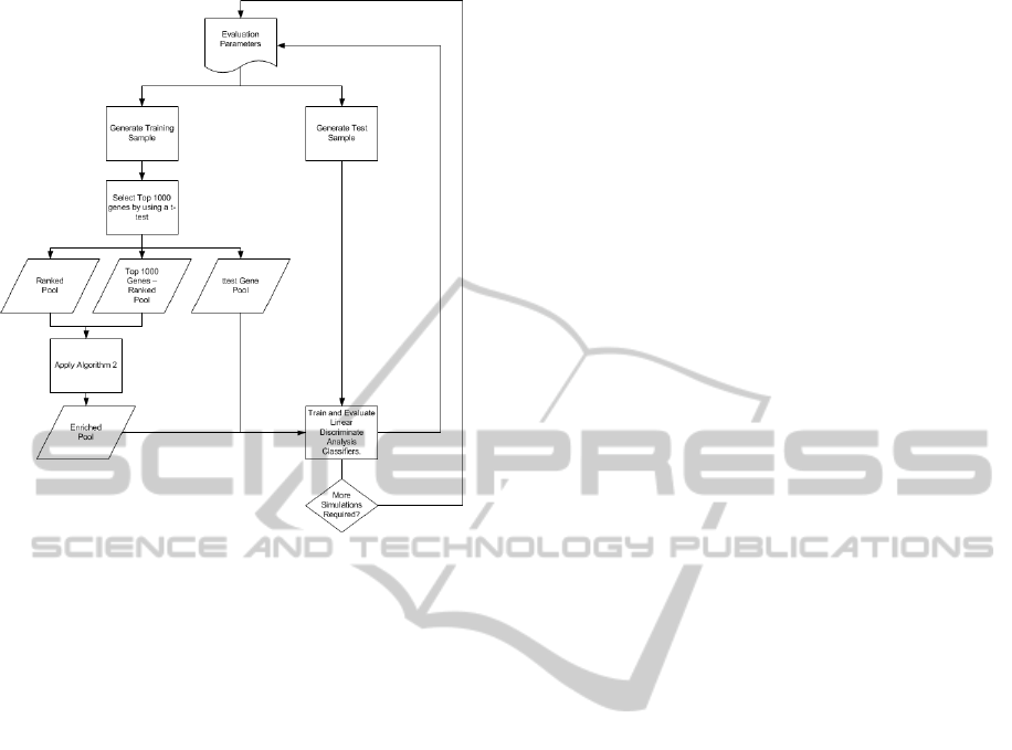
Figure 2: Above is the evaluation part of our simulation.
First the evaluation parameters are input. Next, a training
sample is generated, and the top 1000 genes are selected
using a t-test and input into the top1000ttest pool. The
top 2r genes from the top1000ttest pool are put into the
ttestPool. The top1000ttest genes set is then partitioned
into two groups the top r genes (rankedPool) and the rest of
the genes (top1000ttest − rankedPool). Algorithm 2 uses
the rankedPool to create the enrichelPool. Next, two clas-
sifiers are trained, one using the enrichedPool genes, and
one using the ttestPool genes. Both classifiers are evalu-
ated on a test sample. The process repeats ten times for a
given set of parameters.
Figure 1 diagram captures the preprocessing steps
performed on the data. The first step of the prepro-
cessing algorithm is to load GO and GOA into mem-
ory. We used the 3/1/2011 (mm/dd/yyyy) and the
3/8/2011 versions of GO and GOA. Next we precom-
pute the information content and ancestors for all the
GO terms and construct a look-up table and find the
distinct genes out of 18,141 genes in the human GOA
file. Finally, Algorithm 1 is used to define the “dis-
eased” class’s parameters. The input parameters used
for Algorithm 1 were α = 100, β = 1 and γ = 1. All
the steps for preprocessing and evaluation are limited
to only the biological process ontology. Since α is a
lower bound on the number of genes, Algorithm 1 cre-
ated a subset of genes such that |di f f Genes| = 112.
This is roughly 0.62% of the total number of genes.
After di f f Genes is calculated, the evaluation part,
see Figure 2, of the simulation can be conducted. The
first step of the evaluation procedure is to shift the
means of the“diseased” class’ features in di f f Genes
(112 out of 18,141 genes) from zero to δ and gen-
erate a training sample of size 2s, where each class
gets s samples. Next, detect the top 1000 genes
via the absolute value of the t-test (top1000ttest).
After that, construct a pool (rankedPool) consist-
ing of the top r genes, a pool consisting of all of
the top 1000 t-test genes except for the top r genes
(otherPool), and a pool consisting of the top 2r genes
(ttestPool). Subsequently we apply Algorithm 2 to
create the enrichedPool. The enrichedPool contains
the rankedPool genes in addition to the r most se-
mantically similar genes to the rankedPool genes.
The size of the |enrichedPool| = 2r. Next, we train
two Linear Discriminate Analysis (LDA) classifiers,
one using the ttestPool genes and one using the
enrichedPool genes. Finally, evaluate the classifiers
on a test set consisting of 400 test patterns, where 200
test patterns are from the “healthy” class, and 200 test
patterns are from the “diseased” class. The previous
evaluation steps count as one simulation. For a given
set of parameters, conduct ten simulations and com-
pute the mean accuracy for the classifiers for each
simulation. The simulations were repeated for var-
ious sample sizes, δ values, and rankedPool sizes.
The sample sizes s per class we chose to use were
{10, 20, 30, 40, 50, 60, 70, 80, 90, 100}. The δ values
for the “diseased” class were {.25, .5, .75}. For δ of
.25 we decided to go up to 200 for the sample size,
because the mean difference in accuracy between the
enriched pool LDA classifier and the t-test pool LDA
classifier was still increasing at 100. The ranked pool
sizes r we chose were {10, 20, 40}.
Algorithm 2 is based on the enrichment algorithm
presented in (Papachristoudis et al., 2010). There are
a few important changes this algorithm that we need
to point out. First, ensuring that the similarity of
genes in simPool have semantic similarity ≥ γ induces
some potential bias if the |simPool| < r, because the
size of the enrichedPool can not be increased to 2r.
This has the effect of making some of the pool sizes
slightly smaller in rare cases, during the experimen-
tation. Whenever the enrichedPool could not be in-
creased to 2r, we reduced the size of the ttestPool so
it was the same size as the enrichedPool. This was
done to reduce the effects of this bias. We discuss
how many simulations had this problem in the results
section. In general, to remove the bias one could re-
duce the γ term in Algorithm 2.
3 RESULTS AND DISCUSSION
In this section, we present our results and discuss our
interpretation. One interesting observation is that the
KDIR 2011 - International Conference on Knowledge Discovery and Information Retrieval
298

Algorithm 2: Enrichment Algorithm.
% rankedPool the r top t-test genes
% otherPool = top1000ttest − rankedPool
% similarity[i] = 0 ∀i ∈ otherPool
% γ does not have to be the same as Algorithm 1
for all geneR ∈ rankedPool do
goidsR = {g :g is annotated to geneR in GOA,
and g is a biological process ontology}
for all geneO ∈ otherPool do
goidsO = {g :g is annotated to geneO in GOA,
and g is a biological process ontology}
sim
o
= sim
MAX
(goidsR, goidsO)
if similarity[o] < sim
o
then
similarity[o] = sim
o
end if
end for
end for
simPool = {g : similarity[g] ≥ γ}
% sort simPool in descending order by similarity
% and then in descending order by the
% absolute value of the t-test.
sort(simPool, similarity, top1000ttest)
enrichedPool = rankedPool ∪ {g : g’s index in
simPool ≤ r}
return enrichedPool
mean difference in LDA classification accuracy be-
tween the classifier trained using the enrichedPool
genes and the classifier trained using the ttestPool
genes seems to be represented by a convex-like curve
that is shifted based on the size of δ. As δ increases
the peak of the convex-like curve shifts to the left.
As δ decreases the peak of the convex function shifts
to the right. For example, when δ = .25 the greatest
mean difference between the enrichedPool classifier
and the ttestPool classifier occurs at a sample size of
100. When δ = .5, the peak occurs at a sample size of
30, and when δ = .75 the peak occurs at a sample size
of 10. The sharpness of the curve seems to increase as
δ increases, and decrease as δ decreases. One consis-
tent trend observed is that after the peak difference in
accuracy is reached the difference in accuracy grad-
ually goes to zero or lower. What this means is us-
ing statistical properties of the data set is as good or
superior to using background knowledge in addition
to statistical properties when the sample size is large
enough. In Figures 3 to 7, we present this in three sub-
plots. The first subplot shows the difference in classi-
fication accuracy between the LDA classifiers trained
using the enrichedPool and the ttestPool genes re-
spectively. At each sample size per class the simu-
lations was repeated ten times, and the difference in
accuracy is the difference between the average classi-
fication accuracy of the ten simulations. The horizon-
tal axis shows the number of samples per class used
for training. A 95% confidence interval is shown at
each sample size. These confidence intervals do not
have any correction for multiple testing. The second
subplot shows the average accuracy of the classifiers
over the sample sizes. The third subplot shows the
number of true positive genes that are included in the
enrichedPool, the ttestPool, and the rankedPool.
Figure 3: The upper panel shows the difference in LDA
classification accuracy between the enrichedPool and the
ttestPool when δ = .25 and the pool sizes where 40. The
middle panel shows the actual LDA classification accura-
cies, and the lower panel shows the average number of true
positives detected for the enrichedPool, the ttestPool, and
the rankedPool.
With δ = .25 and rankedPool = ttestPool = 40 we
have a gradual convex like curve, see Figure 3, for the
difference between the accuracy of the LDA classi-
fiers. The greatest difference in accuracy occurs when
the training sample size is 180 per class. The differ-
ence seems to be reducing from 180 to 200 samples
per class.
The rankedPool did not detect many true positives
when the sample size per class was small. This means
Algorithm 2 was not able to add many useful genes
from GO. After the number of true positives reaches
about five, the enrichedPool adds many useful genes.
There were a total of 200 simulations, ten for
each training sample size. Fifteen out of the 200
simulations, the enrichedPool size could not be in-
creased to 40, because there were not enough genes
with a semantic similarity equal to one to the genes
in the rankedPool. If |enrichedPool| < 40 then
the |ttestPool| was adjusted to the same size as the
enrichedPool. All the fifteen simulations where the
|enrichedPool| < 40 occurred when the training sam-
GENE ONTOLOGY BASED SIMULATION FOR FEATURE SELECTION
299

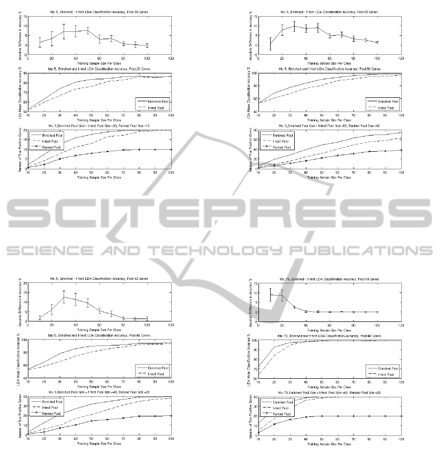
Figure 4: The upper panel shows the difference in LDA
classification accuracy between the enrichedPool and the
ttestPool when δ = .5 and the pool sizes where 20. The
middle panel shows the actual LDA classification accura-
cies, and the lower panel shows the average number of true
positives detected for the enrichedPool, the ttestPool, and
the rankedPool.
Figure 5: The upper panel shows the difference in LDA
classification accuracy between the enrichedPool and the
ttestPool when δ = .5 and the pool sizes where 40. The
middle panel shows the actual LDA classification accura-
cies, and the lower panel shows the average number of true
positives detected for the enrichedPool, the ttestPool, and
the rankedPool.
ple size per class was less than or equal to 100.
When the pool size is 20 and δ = .5, see Figure 4,
the convexity of the difference curve becomes more
apparent. The enrichedPool seems to do best in the
range of 30 to 50 training samples per class. In this
range, the rankedPool had five to eight true positives
out of ten. From 70 training samples per class and
Figure 6: The upper panel shows the difference in LDA
classification accuracy between the enrichedPool and the
ttestPool when δ = .5 and the pool sizes where 80. The
middle panel shows the actual LDA classification accura-
cies, and the lower panel shows the average number of true
positives detected for the enrichedPool, the ttestPool, and
the rankedPool.
Figure 7: The upper panel shows the difference in LDA
classification accuracy between the enrichedPool and the
ttestPool when δ = .75 and the pool sizes where 40. The
middle panel shows the actual LDA classification accura-
cies, and the lower panel shows the average number of true
positives detected for the enrichedPool, the ttestPool, and
the rankedPool.
on, the rankedPool contained all genes that were true
positives. From a training sample size of 80 to 100 per
class, the number of true positives in the enrichedPool
and the ttestPool were 20, which is the most they
could have because the pool size was 20. So, it is
no surprise that the LDA accuracy was nearly identi-
cal at about 85%. When the training sample size per
KDIR 2011 - International Conference on Knowledge Discovery and Information Retrieval
300

class was less than 20, the rankedPool did not have
many true positives genes, so Algorithm 2 could not
add many useful genes. The number of simulations
with bias was three out of 100.
Figure 5 shows what happens when the pool size
is 40 genes for the enrichedPool and the ttestPool.
The subplots are very similar to Figure 4’s subplots,
but the peak of the difference subplot is higher. The
convexity of the difference curve is created by the
rankedPool not detecting many true positives with
small sample sizes initially. In the mid range about
half the genes in the rankedPool are true positives and
in this range the enrichedPool helps significantly. As
the sample size increases the t-test detects more and
more true positives. It seems when a pool of genes has
around 30 or so true positives, the increase in classi-
fication accuracy is minimal when adding more true
positives. The bias was two simulations out of 100.
When the pool size was increased to 80 (Figure 6)
for the enrichedPool and the ttestPool the height of
the difference curve is lowered slightly, the curve is
broader and falls off slower. When the training sam-
ple size per class is ten the enrichedPool makes no
improvement because the rankedPool did not have
many significant genes. In the range of 80 to 100
training samples per class the accuracy of the clas-
sifiers are approaching 100%. The number of simula-
tions with bias was three out of 100.
In Figure 7 where δ = .75, the difference curve is
shifted to the left. The rankedPool contained enough
true positives when the training sample size was less
than 30, so that Algorithm 2 could add useful genes
to the enrichedPool. This made the difference in ac-
curacy much better than the ttestPool in this range.
When the sample size increases out of this range the
accuracy of the LDA classifiers approach 100%, thus
there was not much difference in accuracy. There was
no bias in any runs for this simulation set.
4 SUMMARY AND
CONCLUSIONS
In this paper we conducted a simulation to investigate
the amount of improvement GO and GOA can con-
tribute to gene expression classification accuracy. We
devised an algorithm that defines a group of related
genes di f f Genes in GO. A standard multivariate nor-
mal distribution was used to represent a “healthy” and
a “diseased” class, but the “diseased” class had the
means of the genes in di f f Genes shifted from 0 to δ.
Our simulation compared the accuracy of two LDA
classifiers. One classifier trained using the top ranked
genes as determined by a t-test, and the other classifier
was trained using half of the top ranked t-test genes
and half the genes selected by computing the genes
with highest semantic similarity to the top ranked t-
test genes in GO. We found in our simulation that us-
ing semantic similarity in GO in conjunction with a
t-test improves classification accuracy over the use of
only a t-test, but it is only over a limited range and de-
pends on the parameter δ. When δ = .25 there seems
to be a significant improvement in accuracy when the
training sample size is over 50 per class. When δ = .5,
there is a significant improvement when the training
sample size is over 20 per class, however, this increase
gradually reduces. When δ = .75 there is a signifi-
cant improvement in accuracy when the sample size
per class is less than 30. This work further validates
SoFoCles (Papachristoudis et al., 2010), and lays the
ground work for further investigation of linking this
simulation to real gene expression data.
REFERENCES
Ashburner, M. (2000). Gene ontology: Tool for the unifica-
tion of biology. Nature Genetics, 25:25–29.
Asyali, M. H., Colak, D., Demirkaya, O., and Inan, M. S.
(2006). Gene expression profile classification: A re-
view. Current Bioinformatics, 1:55–73.
Baldi, P. and Long, A. D. (2001). A Bayesian framework for
the analysis of microarray expression data: regular-
ized t -test and statistical inferences of gene changes.
Bioinformatics, 17(6):509–519.
Barrell, D., Dimmer, E., Huntley, R. P., Binns, D., ODono-
van, C., and Apweiler, R. (2009). The GOA database
in 2009-an integrated Gene Ontology Annotation re-
source. Nucleic Acids Research, 37(suppl 1):D396–
D403.
Ben-Dor, A., Bruhn, L., Friedman, N., Nachman, I.,
Schummer, M., and Yakhini, Z. (2000). Tissue classi-
fication with gene expression profiles. In Proceedings
of the fourth annual international conference on Com-
putational molecular biology, RECOMB ’00, pages
54–64, New York, NY, USA. ACM.
Bo, T. and Jonassen, I. (2002). New feature subset selec-
tion procedures for classification of expression pro-
files. Genome Biology, 3(4).
Bontempi, G. (2007). A blocking strategy to improve
gene selection for classification of gene expression
data. Computational Biology and Bioinformatics,
IEEE/ACM Transactions on, 4:293–300.
Breitling, R., Armengaud, P., Amtmann, A., and Herzyk,
P. (2004). Rank products: a simple, yet powerful,
new method to detect differentially regulated genes
in replicated microarray experiments. FEBS Letters,
573(1-3):83 – 92.
Campo, J. L. S., Segura, V., Podhorski, A., Guruceaga, E.,
Mato, J. M., Mart
´
ınez-Cruz, L. A., Corrales, F. J., and
Rubio, A. (2005). Correlation between gene expres-
GENE ONTOLOGY BASED SIMULATION FOR FEATURE SELECTION
301

sion and GO semantic similarity. IEEE/ACM Trans.
Comput. Biology Bioinform, 2(4):330–338.
Ding, C. and Peng, H. (2003). Minimum redundancy fea-
ture selection from microarray gene expression data.
In Bioinformatics Conference, 2003. CSB 2003. Pro-
ceedings of the 2003 IEEE, pages 523 – 528.
Duan, K.-B., Rajapakse, J., Wang, H., and Azuaje, F.
(2005). Multiple svm-rfe for gene selection in cancer
classification with expression data. NanoBioscience,
IEEE Transactions on, 4(3):228 –234.
Dudoit, S., Fridlyand, J., and Speed, T. P. (2002). Compar-
ison of discrimination methods for the classification
of tumors using gene expression data. Journal of the
American Statistical Association, 97(457):77.
Efron, B., Tibshirani, R., Storey, J. D., and Tusher, V.
(2001). Empirical Bayes Analysis of a Microarray
Experiment. Journal of the American Statistical As-
sociation, 96(456):1151–1160.
Fox, R. and Dimmic, M. (2006). A two-sample bayesian
t-test for microarray data. BMC Bioinformatics,
7(1):126.
Furey, T. S., Cristianini, N., Duffy, N., Bednarski, D. W.,
Schummer, M., and Haussler, D. (2000). Support vec-
tor machine classification and validation of cancer tis-
sue samples using microarray expression data. Bioin-
formatics, 16(10):906–914.
Golub, T. R., Slonim, D. K., Tamayo, P., Huard, C., Gaasen-
beek, M., Mesirov, J. P., Coller, H., Loh, M. L., Down-
ing, J. R., Caligiuri, M. A., Bloomfield, C. D., and
Lander, E. S. (1999). Molecular Classification of Can-
cer: Class Discovery and Class Prediction by Gene
Expression Monitoring. Science, 286(5439):531–537.
Jafari, P. and Azuaje, F. (2006). An assessment of recently
published gene expression data analyses: reporting
experimental design and statistical factors. BMC Med-
ical Informatics and Decision Making, 6(1):27.
Kumar, P. V., Vinodh, K., An, M., and Elia, P. (2001). The
gene ontology consortium: Creating the gene ontol-
ogy resource: design and implementation. Genome
Res, pages 1425–1433.
Leung, Y. and Hung, Y. (2010). A multiple-filter-multiple-
wrapper approach to gene selection and microarray
data classification. Computational Biology and Bioin-
formatics, IEEE/ACM Transactions on, 7(1):108 –
117.
Li, L., Weinberg, C. R., Darden, T. A., and Pedersen, L. G.
(2001). Gene selection for sample classification based
on gene expression data: study of sensitivity to choice
of parameters of the GA/KNN method. Bioinformat-
ics, 17(12):1131–1142.
Pan, W. (2003). On the use of permutation in and the
performance of a class of nonparametric methods to
detect differential gene expression. Bioinformatics,
19(11):1333–1340.
Papachristoudis, G., Diplaris, S., and Mitkas, P. A. (2010).
Sofocles: Feature filtering for microarray classifica-
tion based on gene ontology. Journal of Biomedical
Informatics, 43(1):1 – 14.
Paul, T. K. and Iba, H. (2009). Prediction of cancer class
with majority voting genetic programming classifier
using gene expression data. Computational Biol-
ogy and Bioinformatics, IEEE/ACM Transactions on,
6(2):353–367.
Pesquita, C., Faria, D., Falco, A. O., Lord, P., and Couto,
F. M. (2009). Semantic similarity in biomedical on-
tologies. PLoS Comput Biol, 5(7):e1000443.
Resnik, P. (1995). Using information content to evaluate
semantic similarity in a taxonomy. In Proceedings of
the 14th international joint conference on Artificial in-
telligence - Volume 1, pages 448–453, San Francisco,
CA, USA. Morgan Kaufmann Publishers Inc.
Saeys, Y., Inza, I. n., and Larra
˜
naga, P. (2007). A review of
feature selection techniques in bioinformatics. Bioin-
formatics (Oxford, England), 23(19):2507–2517.
Saraswathi, S., Sundaram, S., Sundararajan, N., Zimmer-
mann, M., and Nilsen-Hamilton, M. (2011). Icga-pso-
elm approach for accurate multiclass cancer classifica-
tion resulting in reduced gene sets in which genes en-
coding secreted proteins are highly represented. Com-
putational Biology and Bioinformatics, IEEE/ACM
Transactions on, 8(2):452–463.
Seco, N., Veale, T., and Hayes, J. (2004). An intrinsic
information content metric for semantic similarity in
wordnet. In de M
´
antaras, R. L. and Saitta, L., editors,
ECAI, pages 1089–1090. IOS Press.
Speed, T. P., editor (2003). Statistical Analysis of Gene Ex-
pression Microarray Data. Chapman and Hall.
Statnikov, A., Aliferis, C. F., Tsamardinos, I., Hardin, D.,
and Levy, S. (2005). A comprehensive evaluation
of multicategory classification methods for microar-
ray gene expression cancer diagnosis. Bioinformatics,
21(5):631–643.
Thomas, J. G., Olson, J. M., Tapscott, S. J., and Zhao,
L. P. (2001). An Efficient and Robust Statistical Mod-
eling Approach to Discover Differentially Expressed
Genes Using Genomic Expression Profiles. Genome
Research, 11(7):1227–1236.
Wang, L., Chu, F., and Xie, W. (2007). Accurate
cancer classification using expressions ofvery few
genes. IEEE/ACM Trans. Comput. Biology Bioinform,
4(1):40–53.
Wang, Y., Tetko, I. V., Hall, M. A., Frank, E., Facius, A.,
Mayer, K. F., and Mewes, H. W. (2005). Gene selec-
tion from microarray data for cancer classification–a
machine learning approach. Computational Biology
and Chemistry, 29(1):37 – 46.
Xu, T., Du, L., and Zhou, Y. (2008). Evaluation of GO-
based functional similarity measures using S. cere-
visiae protein interaction and expression profile data.
BMC Bioinformatics.
Yeoh, E.-J., Ross, M. E., Shurtleff, S. A., Williams, W., Pa-
tel, D., Mahfouz, R., Behm, F. G., Raimondi, S. C.,
Relling, M. V., Patel, A., Cheng, C., Campana, D.,
Wilkins, D., Zhou, X., Li, J., Liu, H., Pui, C.-H.,
Evans, W. E., Naeve, C., Wong, L., and Downing, J. R.
(2002). Classification, subtype discovery, and pre-
diction of outcome in pediatric acute lymphoblastic
leukemia by gene expression profiling. Cancer Cell,
1(2):133 – 143.
KDIR 2011 - International Conference on Knowledge Discovery and Information Retrieval
302