STUDY ON THE LONG-TERM INCENTIVE MECHANISM

OF THE LARGE-SCALE DREDGING PROJECT

Bin Zhou and Zigang Zhang

Huazhong University of Science and Technology, Wuhan 430074, Hubei Province, China

Keywords: Dredging project, Principal-agent, Long-term income, Incentive mechanism.

Abstract: Through the principal-agent theory and game theory, this article has established the long-term income

model of the large-scale dredging project, which has obtained the solution of the long-term incentive model,

analyzed the impact of the dynamic consistency as well as pledge and negotiating cost to incomes of the

principal and agent by means of increasing different constraint conditions. Furthermore, the study also

shows that the long-term incentive model can provide the agent with stronger incentive.

1 INTRODUCTION

The incentive is essential for the management, and

the principal-agent theory is widely applied for the

analysis on the incentive problem. And, the

principal-agent theory deems the management

problem as the fact that how the principal designs

the incentive mechanism to seduce the agent to take

behaviors optimum to the principal from his own

interests. In 1981, Lazear put forward the game

theory, and he thought that the large salary gap can

reduce the monitoring cost, seduce efforts of the

agent, and highly motivate the consistent interests of

the principal and the agent. (Lazear E, Rosen S.,

1981). Furthermore, Holmstrom & Milgrom put

forward the output share incentive mechanism that

the purely selfish and risk-neutral principal shall

employ the agent with the jealousy and pride

preference and risk avoidance. (Holmstrom B,

Milgrom P., 1987). And, Aoki pointed out that, the

long-term employment can motivate the agent to

accumulate human capitals special for the enterprise.

(Aoki, M.,1988). Also, Yong Zhang established the

two-stage model for the manager, that is the long-

term and short-term income incentives as well as

obtained solutions and analyzed relevant

conclusions. (Yong Zhang. 2004). The study of

Debing Ni revealed that the optimal sharing

proportion will increase along with the increased

effort cost of the agent while reduce along with the

increased expected growth rate of the market price

and effort output. (Debing Ni and Xiaowo Tang.,

2005). Besides, Zongjun Wang obtained the optimal

income combination of the manager through the

long-term and short-term incentive models.

(Zongjun Wang, Chongshuai Qian, and Tian Xia,

2008). Lijun Li studied the problem of how to

motivate the producer to reduce costs as well as

pointed out the cost difference between the

asymmetric information and the symmetric

information, namely the incentive cost; only if the

agent shares the cost-saving income, can the

principal realize his expected income; in the premise

of incomplete and asymmetric information of the

dredging project. (Lijun Li, Xiaoyuan Huang, etc.,

2003). Bin Zhou put forward the relationship

between the agent’s incentive coefficient and the

project cost; that is, the higher the agent’s incentive

coefficient, the lower the project cost; in addition to

the above, it also established the incentive

mechanism based on the equity preference. (Bin

Zhou, Zigang Zhang, 2010).

Above scholars have studied the income of the

manager from different views; however the actual

income of the agent will be restricted by numerous

kinds of factors. This article, from the long-term

incentive view, has corrected relevant study

assumptions, increased the long-term incentive

constraint and the agent’s capability constraint, and

compared the impact of the long-term and short-term

incentives to the agent’s income to make the model

be close to actual conditions and obtain

corresponding conclusions.

574

Zhou B. and Zhang Z..

STUDY ON THE LONG-TERM INCENTIVE MECHANISM OF THE LARGE-SCALE DREDGING PROJECT.

DOI: 10.5220/0003591905740580

In Proceedings of the 13th International Conference on Enterprise Information Systems (PMSS-2011), pages 574-580

ISBN: 978-989-8425-56-0

 2011 SCITEPRESS (Science and Technology Publications, Lda.)

2 MODELING

In order to facilitate the study, following

assumptions are introduced:

Assumption1: Both the principal and the agent

pursue maximizing own benefits.

Assumption 2: In a certain period, the agent’s

current income will be related to that of previous

period, and his ability will be enhanced along with

the increased service year.

Assumption 3: The agent’s capability can be

applied to pursue the short-term income and long-

term income, and the required negotiating cost for

signing one contract is

Supposing the payment made by the principal to

the agent is

vky =

Ni ,...,2,1

; i refers to the

stage

i project, and the total of the stage

project is

cube (earthwork); the bid award price of the

unilateral dredged soil of the stage

project is

yuan/cube; the project agent’s oil consumption

and material consumption of the stage

are

yuan/cube, with the fixed cost of

yuan/hour; the

income of the stage

project is

yuan/cube; the

principal’s income of the stage

project is

yuan/cube; the payment made by the principal to

the agent of the stage

i project is

yuan/cube.

When the agent’s effort cost is

)(ac

yuan/hour,

refers to the agent’s payroll in the competitive

market; the agent’s income of the stage

i project is

yuan/cube; when the maximum rated hourly

output of the engineering ship applied by the agent

cube/hour, the output when the project income

is zero; namely the critical output is

cube /hour.

According to above assumptions, the model to

maximize the principal’s income is as follows:

∑∑

−=

vyvvMax

)]([

(1)

0])([

≥−−=

∑∑

iii

ctxpv

(2)

∑∑

≥−=

acvyv

0)]()([

(3)

∑

≤

kk ≥

pp = )

(4)

∑∑

≥−=

Nyacvyv

)]()([

))(

(

−

−−

−=

48.0=

(5)

Ni ,...,2,1

In the model, the objective function (1) formula

means the principal’s utility function of the stage N

project; constraint (2) means the total utility function

of the stage N project; constraint (3) means the

agent’s utility function of the stage N project; when

the agent pursues maximize his own utility, the

formula is objective function, and the formula (1)

which is larger than or equals to 0 is the constraint

condition; the (4) formula is the rigid constraint

condition, when the agent enhances the hourly

output to the rated output, the game pricing incentive

coefficient is 1/2, and the incentive coefficient of the

stage N project will not be larger than the sum of N

short-term game incentive coefficients; or else, the

principal is inclined to sign the short-term contract.

According to the assumption 2, when the agent is

engaged in some work for a long time, his capability

will be improved gradually; therefore, his income

shall be increased correspondingly; the constraint (5)

expresses that, the income of the long-term contract

signed by the agent shall be higher than that of the

short-term contract;

y refers to the income of the

short-term game pricing formula.

3 MODEL SOLUTION AND ITS

ANALYSIS

3.1 Solution to Maximize the

Principal’s Income in Stage N

Firstly, give up the constraint (4) and the constraint

(5), and directly solve the problem of maximizing

the principal’s income in the stage N

Establish Lagrange function and obtain the

agent’s reaction function in the stage N:

Derive the

,,...,,

21 N

NNN

kkk

in turn and

eliminate

, including

−

Ni ,...3,2=

(6)

STUDY ON THE LONG-TERM INCENTIVE MECHANISM OF THE LARGE-SCALE DREDGING PROJECT

575

The principal knows the agent’s reaction

function in the stage N; then, the principal’s optimal

incentive coefficient in the stage I is as follows

aNa

NNi

ccvkvkv ...)1...()1(

++−+−=

∑

(7)

Substitute the (7) formula by (6); make the first

derivation to

, and make the derivative as 0,

including

−

−=

(8)

∂

>0 ,

∂

<0, when

pp =

, make

; that is, when the agent increases the output

to the rated one of the ship, the corresponding

incentive coefficient will reach the maximum

value

, including:

)(

))(

(

−

−−

−=

(9)

Viewing from the (9) formula, the

value shall

be larger than 0, which shall be related to the

validity of the contract signed between the principal

and the agent.

Making

(10)

))(1(

)(1

ppNN

−+

−

−=

pp >

(11)

Such formula meets the monotonic increasing

requirements of the incentive coefficient

k to the

hourly output

as well as demands that the second

derivative shall be smaller than 0. As

)1(

−=

∂

fails to meet conditions of the

assumption (2), this formula shall be converted.

Supposing that the agent increases the hourly output

p in whole N cooperation periods of the

principal and the agent, the agent’s optimal incentive

coefficient in the stage I is

. In addition to

the above, with the increased cooperation period, the

incentive coefficient will increase till

in the

last period. During N stages of the contract, the

agent’s incentive coefficient will be increased by

for each increasing cooperation. Therefore, the

agent’s optimal incentive coefficient shall be as

follows:

Table 1: Calculation Sheet of the Principal’s and Agent’s

Income when p=p

m..

1 2 3 … N

−N

…

According to above reasonings, the (11) formula

can be rewritten as

3.2 Solution to Maximize the Agent’s

Income in Stage N

Firstly, give up the constraint (4) and the constraint

(5), and directly solve the problem of maximizing

the agent’s income in the stage N. here, the agent’s

income is the objective function, and the principal’s

income is larger than 0, which is the participation

constraint.

Establish Lagrange function and obtain the

principal’s reaction function in the stage N,

including:

Derive the

,,...,,

21 N

NNN

kkk in turn and

eliminate

, including

)1(1

−

−−=

Ni ,...3,2=

(13)

The agent knows the principal’s reaction

function in the stage N; then, the agent’s optimal

incentive coefficient in the stage I is as follows

Substitute the (13) formula by (3); make the first

derivation to

, including:

)(

ppN

−

−−=

(14)

∂

>0 ,

∂

<0, when

pp =

k will be

maximum; therefore,

ppc

−=

; that is, when the

))(2)(1(1

ppiNiN

−−+−+

−

−+

(12)

ICEIS 2011 - 13th International Conference on Enterprise Information Systems

576

agent increases the output to the rated one of the

ship, the corresponding incentive coefficient will

reach the maximum value, including:

)(

ppN

−

−−=

(15)

>+=

∂

, which meets the constraint

(2); that is, during the contract period, the agent’s

incentive coefficient will be increased along with the

increased working time. Accordingly, the (15)

formula can be rewritten as:

1=i

)(

)(1

ppi

−

−−=

Ni ,...3,2=

(16)

3.3 Solution of the Long-term Incentive

Model

When both the principal’s income and the agent’s

income are optimal, the optimization solution can be

obtained without the constraint (4) and the constraint

(5). Compare the (12) and (16) formulas, the agent’s

incentive coefficient will meet

0,0

∂

; that

is, the agent’s incentive coefficient will be increased

along with the increased working time. The long-

term cooperation will be good to the agent; however

the principal’s long-term optimization is not the

same as the agent’s long-term optimization;

accordingly, the feasible solution of the long-term

optimization is between the principal’s long-term

income optimization solution and the agent’s long-

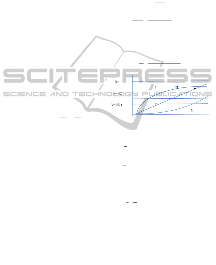
term income optimization solution. Viewing from

the figure 1, we find out that the feasible solution is

located in the area between line I and line III.

However, after increasing the constraint (4) and

constraint (5), the principal’s income optimization

solution (12) formula and the agent’s income

optimization solution (16) formula can’t meet the

constraint (4) constraint (5); therefore, solutions

meeting all constraint conditions of the long-term

incentive shall be obtained

. According to the

constraint conditions (4), when

pp =

121

...

kkkk >>>>

−

, supposing

])1(1[

kik

−+=

Ni ,...,2,1=

, then

]

1[2

−

≤

(17)

According to the agent’s incentive coefficient

solution when the principal income is optimal, when

(18)

Making

]

1[2

−

; therefore,

when

, then, when

ppp ≤≤

))(1(

)(

ppNN

ppi

−+

−

−=

(19)

Figure 1: Comparison Chart of the Agent’s Incentive

Coefficient.

—Total incentive coefficient of the project

—Agent’s incentive coefficient line in the

dynamic game pricing formula (

pp =

)

rk −=

—Agent’s incentive coefficient after

deducting the negotiating cost in the dynamic game

pricing formula (

)

I---Agent’s incentive coefficient line when the

long-term contract agent is optimal (

pp =

−−=

Ni ,...2,1

II---Agent’s long-term incentive coefficient line

(

Ni ,...2,1

III---Agent’s incentive coefficient line when the

long-term contract principal is optimal (

pp =

−+

Ni ,...2,1

STUDY ON THE LONG-TERM INCENTIVE MECHANISM OF THE LARGE-SCALE DREDGING PROJECT

577

3.4 Comparative Analysis on Three

Solutions

3.4.1 Long-term and Short-term Dynamic

Consistency

Determine the agent’s incentive coefficient based on

the maximization of the principal’s long-term

income; namely the (12) formula.

Without considering discounts, suppose that the

agent tries to increase the output of the ship to the

rated one during the cooperation period, the sum of

incentive coefficients of three stages shall be

=++=

∑

and agent’s total incentive

coefficient sum during 30-year career shall be

130

However, if the agent and the principal sign the 30-

year contract, the agent’s 30-year incentive

coefficient sum shall

9.2

...

≈++++=

∑

. Therefore, the

longer contract period will be more beneficial to the

principal; however, for the agent, the higher

expectations for the future, the shorter-term contract

will be.

Determine the agent’s incentive coefficient based

on the maximization of the agent’s long-term

income; namely the (16) formula or the comparison

between 3-period and 30-period. Without

considering discounts, the incentive coefficient sum

of three-period contract is:

=++=

∑

;

that of ten 3-period contracts within 30 years is

130

and that of 30-period is:

900

869

841

811

...

>+++++=

∑

Obviously, the long-term contract is more

beneficial to the agent. Under such condition, the

principal will choose to sign the contract with short

cooperation period. Therefore, under these two

conditions, the principal and the agent are in the

bargaining game process; namely, the principal and

agent are dynamically inconsistent in the long-term

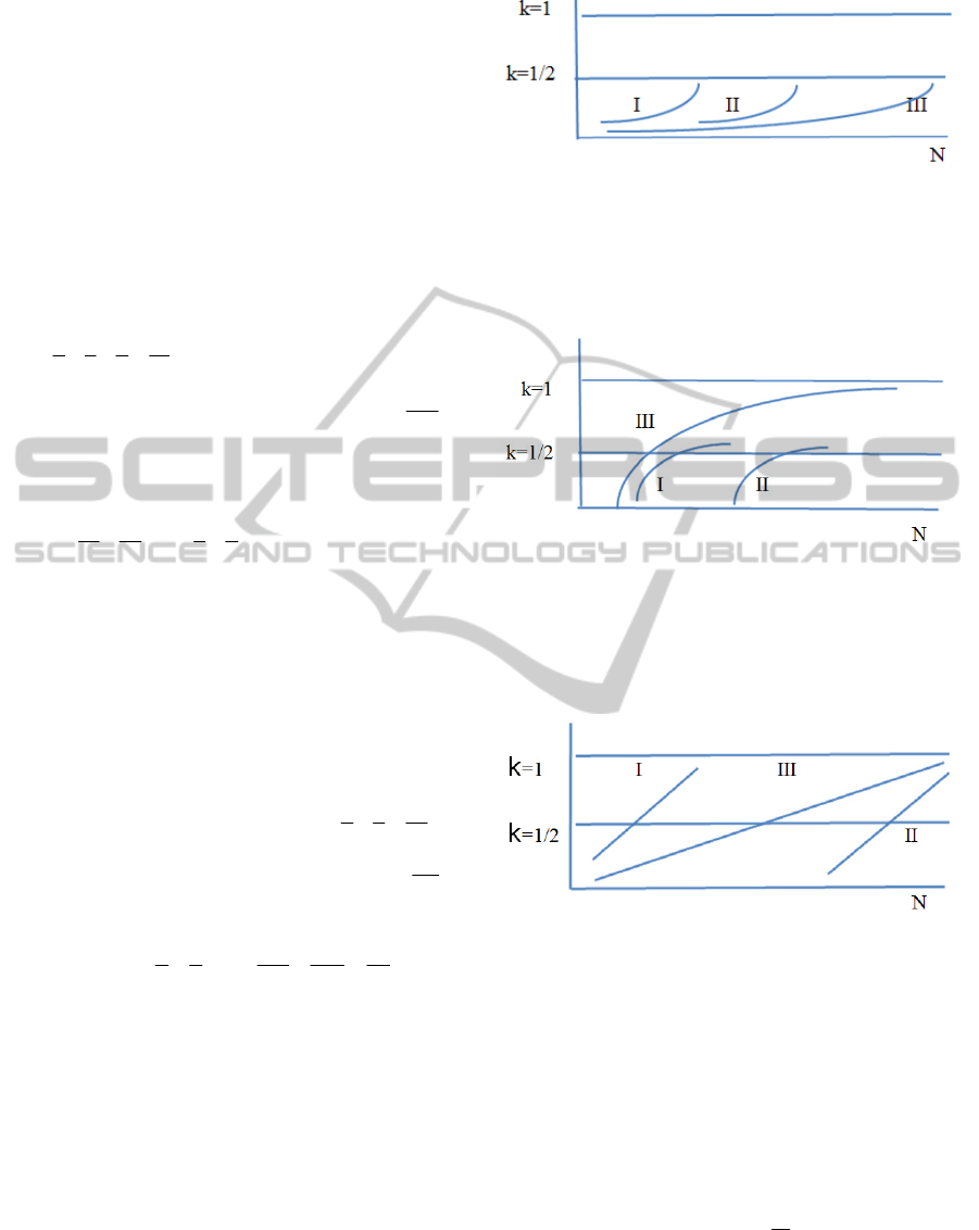
and short-term incomes, see figure 2 [A,B,C].

I, II—Incentive coefficient line of

3,2,1,,3 === ippN

;

III—Incentive coefficient line of

NippN

,...2,1,,30 ===

Figure 2A: Comparison Between the Long-term and

Short-term Incentive Coefficients in the Principal’s Long-

term Income Optimization.

I, II—Incentive coefficient line of

3,2,1,,3 === ippN

III—Incentive coefficient line of

NippN

,...2,1,,30 ===

Figure 2B: Comparison Between the Long-term and

Short-term Incentive Coefficients in the Agent’s Long-

term Income Optimization.

I, II—Incentive coefficient line of

3,2,1,,3 === ippN

III—Incentive coefficient line of

NippN

,...2,1,,30 ===

Figure 2C: Comparison the Long-term and Short-term

Incentive Coefficients in the Long-term Incentive Model.

Determine the agent’s incentive coefficient based

on the long-term incentive model solution; namely

the (19) formula. No matter how long the contract

period is, when the agent tries to increase it to the

rated output

, it can certify that the incentive

coefficient sum meets

∑

; namely the (19)

formula meets the dynamic consistency of the long-

term and short-term incomes of the principal and the

agent.

ICEIS 2011 - 13th International Conference on Enterprise Information Systems

578

3.4.2 Comparison between the Long-term

Income and the Short-term Income

As the long-term optimization solutions of the agent

and the principal can’t meet the dynamic

consistency, it is not a kind of stable solution, which

will change along with both parties’ negotiating

skills. When the principal takes the priority, he

hopes to sign the long-term contract based on his

long-term income optimization; however, the agent

prefers to the dynamic game pricing. When the agent

takes the priority, he hopes to sign the long-term

contract based on his long-term income

optimization; however, the principal prefers to the

dynamic game pricing. Accordingly, the analysis on

the dynamic game pricing and long-term incentive

model solutions will be more significant. Taking the

3 stages as the example, the negotiating cost will not

be considered and the agent’s calculation data in the

3 stages are the same.

The income of 3 contracts signed by the agent

according to the short-term game pricing coefficient

is:

dpctxp

ppp

])([]

)(

))(3

(

)(

−−

−

−−

−=

∫

−+

The agent signs a 3-period contract based on the

long-term incentive model:

)(12

)(

ppii

−

−=

3,2,1,3 == iN

dpctxp

ppp

∫

∑

−+

−−

−

−=

)(

])(][

)(2

)(

dpctxp

ppp

])([]

)(

)(44.0

)(

−−

−

−=−

∫

∑

−+

0])(][

)(2

)(

>−−

−

−+

∫

−+

ppp

dpctxp

3.4.3 Negotiating Cost r

Costs are required for facts that the principal

searches for the agent and the agent signs the

agreement with the principal; compared with the

scale advantages of the principal, the proportion of

the agent’s negotiating cost of its own income will

be higher. As for the agent, if there is no negotiating

cost

, the incentive coefficient of N 1-period

contract is the same as the sum of the incentive

coefficient of the N-period contract. When the

negotiating cost

0>r , and

Nrrk

)

(

−>−

∑

, the

income of the N-period contract will be higher than

that of N 1-period contracts. As for the principal,

though the negotiating cost proportion of the income

is not high, the long-term contract will be more

beneficial.

3.4.4 Pledged Capital w or “Hostage”

When calculating from the figure 1,

∫∫

−=−−=

Nai

dtcvkdtcvkw

)(])

[(

The income of the agent’s first half of the career

which is deducted by the principal has been

compensated in his later half of the career, which

can be deemed as the investment or savings made by

the agent to the principal. Due to the pledged capital,

the agent’s and the principal’s goals are further

harmonized, and if the agent be fired because of

effortless, or lead to the principals’ fewer income;

the agent will also have corresponding loss. And, the

longer the worktime is, the larger the corresponding

loss will be. Accordingly, the long-term contract

incentive to the agent is larger.

4 CONCLUSIONS

From the standpoint of the long-term incentive, the

article has studied the income of the agent of the

large-scale dredging project, established the long-

term incentive model, obtained the optimization

solutions of the principal’s long-term income and the

agent’s long-term income; in addition to the above,

it has obtained the long-term incentive model

solution through increasing various kinds of

constraints (long-term incentive constraint, agent’s

capability constraint, and short-term income

constraint ). The main conclusions cover: I. As for

the principal’s long-term optimization solution and

the agent’s long-term optimization solution; while as

the long-term incentive model solution can meet the

dynamic consistency requirements, it is a kind of

stable solution; II. In the long-term incentive model,

the agent’s long-term income is higher than the

short-term income, which has provided the agent

with stronger incentive; III. If consideration is not

given to the negotiating cost, the sum of the

coefficient of the short-term game price equals to

STUDY ON THE LONG-TERM INCENTIVE MECHANISM OF THE LARGE-SCALE DREDGING PROJECT

579

that of the long-term incentive model. If there is the

negotiating cost, the coefficient sum of the long-

term contract is larger than that of the short-term

contract; accordingly, the long-term contract will be

beneficial to the principal and the agent; IV. As the

existence of the pledge, the objection of the agent

and the principal will be more gradually-consistent.

the agent’s incentive shall be further strengthened;

V. The long-term incentive coefficient is similar to

the seniority pay while the seniority pay also has

differences. The classification of the long-term

incentive coefficient is the sharing proportion of the

project income; thus the principal shall also assess

the agent’s hourly output. When the income of the

project under the management of the agent is lower,

the principal shall not increase the agent’s incentive;

namely, coefficient by years, that is, the interior

promotion system shall be established. After

increasing the constraint, the long-term incentive

model will be more practicable and convenient

operation and application. And, the disadvantage is

that, as the article fails to give the agent capability

classification incentive mode, which shall be further

studied.

REFERENCES

Lazear E, Rosen S. 1981, Rank-order Tournaments As

Optimum Labor Contracts [J]. Journal of Political

Economy, 89(5): 841

∼864.

Holmstrom B, Milgrom P. 1987, Aggregation and linearity

in the provision of intertemporal incentives [J].

Econometrica, 55(2): 303

∼328.

Aoki, M., 1988, Information, Incentives and Bargaining in

the Japanese Economy, Cambridge University Press.

Yong Zhang. 2004, Discussion of the Manager Long-term

and Short-term Income Incentive [J]. Management

Engineering Journal, 18(3): 125

∼127.

Debing Ni and Xiaowo Tang. 2005, Paincipal-agent

Model of the Hard Decision Sharing System of

Agent’s Hard Decision Flexibility Cutting [J].

Management Science Journal, 8 (3): 15

∼23.

Zongjun Wang, Chongshuai Qian, and Tian Xia. 2008

manager long-term and short-term incentive income

model and its optimization study [J] Management

Engineering Journal, Vol.22, No.1,113

∼116.

Lijun Li, Xiaoyuan Huang, etc. 2003, Application of the

Paincipal-agent theory in the Reduced Cost [J].

Industrial Engineering and Management, 4(4): 55

∼58.

Bin Zhou, Zigang Zhang, 2010, Pricing the Cost of

Dredging Engineering Based on the Dynamic Game,

Vol.2 No. 184,

Bin Zhou, Zi Gang Zhang, 2011, Study on Incentive

Mechanism of Large-scale Dredging Project Based on

Fairness Preference [J]. Advanced Materials Research,

Vol.219-220:144

∼150.

ICEIS 2011 - 13th International Conference on Enterprise Information Systems

580