
LINEAR COMPLEXITY STEREO CORRESPONDENCE
From Interpolation to Segment-based Approach
Vilson Heck Junior
Departamento de Ensino, Pesquisa e Extensão, Instituto Federal de Santa Catarina, Lages, SC, Brazil
Marcelo Ricardo Stemmer
Departamento de Automação e Sistemas, Universidade Federal de Santa Catarina, Florianópolis, SC, Brazil
Keywords: Linear Complexity, Stereo Correspondence, Segment-based Approach.
Abstract: This paper presents the work in progress on the enhancement of a stereo correspondence method based on
linear complexity region indexing with an image segmentation method. Such improvement shows itself to
achieve better results (compared to its predecessor) when evaluated on Middlebury Stereo Evaluation,
keeping the computing complexity () of the algorithmic solution. In spite of the better results, this
method still need to solve some issues related to surfaces inclinations. The steps taken to create this
improvement, some stereo correspondence results and evaluations are presented.
1 INTRODUCTION
Perception is an important field on MR (Mobile
Robotics). This field still has a need of solutions’
development, mainly on computer vision (Murray
and Little, 2000). The MR perception can be
performed by several different kinds of passive and
active sensors. This work explores the subfield of
PSV (Passive Stereoscopic Vision) for MR.
For a better understanding, PSV’s classic
processing pipeline is: 1) Calibration; 2)
Rectification; 3) Correspondence; 4)
Reconstruction; 5) Spatial Information Use. Of
course, some applications don’t use this whole
pipeline, but most of them do. In our case, we are
going to assume that we have well defined and
working methods for steps 1, 2, 4 and 5. That sets
our focus to step 3, the Correspondence issue.
In our application scenario, we seek to build
complete 3D maps from the MR environment. We
also aim to recognize 3D objects. When using dense
correspondence, instead of the sparse one, we will
be able to obtain information around solid objects
and walls. These “solid” objects allow us to compute
complete 3D maps, instead of partial 3D maps or
merely 2D maps of the environment. These
constraints led us to choose the dense
correspondence instead of sparse correspondence.
When the MR is operating, it is preferred to use
low cost computing methods for processing all kinds
of information. That preference is either related to
energy saving or to low time processing.
Based on those premises, this work developed a
research on dense correspondence methods. We
started by comparing a LM (Linear Complexity
Method) (low cost computing) - presented at
(Oliveira and Wazlavick, 2005) - with a state-of-the-
art method.
1.1 Middlebury Images
For comparison and evaluation purposes, the method
used in this work is proposed by (Scharstein and
Szeliski, 2002) and (Scharstein and Szeliski, 2003).
The authors of this EM (evaluation method) also
provide a web-based rank, for comparison with
several state-of-the-art methods (Middlebury, 2011).
This approach is widely accepted and used when
comparing stereo correspondence methods.
This EM has 4 (four) most used stereo image
pairs available; each pair has an expected
correspondence result and a name. We have used the
four images in our evaluations, but only the results
for Teddy pair will be shown on this paper as
illustrative results. The pairs’ names are: Teddy,
Tsukuba, Venus and Cones. The Teddy original left
308
Heck Junior V. and Ricardo Stemmer M..
LINEAR COMPLEXITY STEREO CORRESPONDENCE - From Interpolation to Segment-based Approach.
DOI: 10.5220/0003539803080312
In Proceedings of the 8th International Conference on Informatics in Control, Automation and Robotics (ICINCO-2011), pages 308-312
ISBN: 978-989-8425-75-1
Copyright
c
2011 SCITEPRESS (Science and Technology Publications, Lda.)
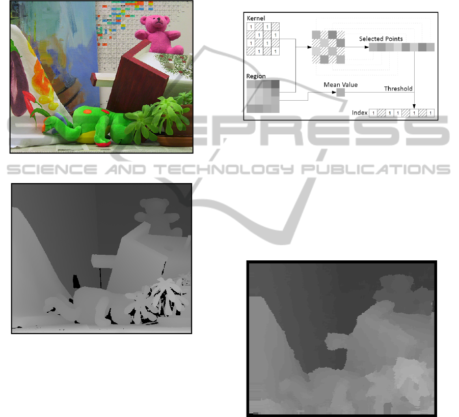
image is shown in Figure 1 and its expected result is
depicted in Figure 2.
There are 3 (three) main evaluations performed
by this EM: 1) nonocc – performs evaluation only
on non-occluded areas; 2) all – performs evaluation
in all areas of the expected result; and 3) disc –
evaluates only “near image edges” areas.
Figure 1: Left image of the Teddy stereo pair.
Figure 2: Expected correspondence result for the Teddy.
2 THE LINEAR APPROACH
The LM was proposed by Oliveira and Wazlavick,
2005 and performs dense stereoscopic
correspondence on linear computing complexity.
That means an algorithmic solution on () and
plays a role on low computing cost. The above-
mentioned method is divided in four basic steps: 1)
Region indexing based on intensities; 2) Wrong
correspondences elimination; 3) Continuity
verification; 4) Disparity map interpolation. The first
three steps generate sparse correspondence results
and step four generates the dense result by
interpolation.
Step 1, region indexing based on intensities, is
described in Figure 3. A Kernel is applied to a
Region to describe a chain of Selected Points. Also,
a Mean Value from the Region is used as reference
on a Binary Threshold procedure over the Selected
Points. The result is a binary Index number, for
finding corresponding regions over the stereo’s
epipolar line.
Figure 3: Indexing operation for LM. Image from
(Oliveira and Wazlavick, 2005).
When applying this LM to the Teddy image,
(Scharstein and Szeliski, 2003), we reach the result
shown in Figure 4. The obtained result for this LM
can be visually compared to the expected result
(Figure 2), where both of them showed similar
disparities to the same regions. The biggest
differences between them (errors) are around the
edges of the image’s objects.
Figure 4: Final result for the linear method on Teddy.
We also applied this method to images Tsukuba,
Venus and Cones and we submitted all the results
taken to EM presented in section 1.1. The EM
results can be found in Table 1.
Despite of the similar result presented in Figure
4, the evaluation’s results in Table 1 report a bad
correspondence between all of the obtained results
against the expected results for all the images.
LINEAR COMPLEXITY STEREO CORRESPONDENCE - From Interpolation to Segment-based Approach
309
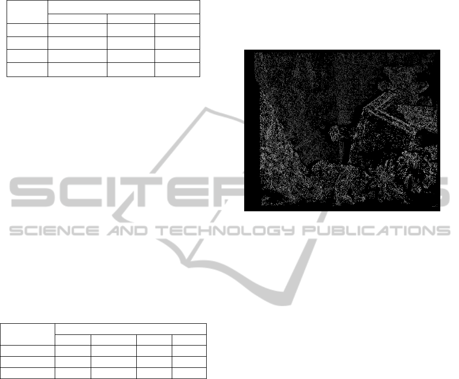
Table 1: Original linear method evaluation (Closer to 0.0
best. Closer to 100.0 worst). Threshold = 2.
Image
Evaluation
nonocc all disc
Tsukuba 94.0 93.4 85.6
Venus 99.8 99.8 97.7
Teddy 100.0 99.5 99.9
Cones 99.7 99.4 99.1
2.1 Sparse Evaluation of Steps
After getting bad scores from the LM’s final result,
we studied the sub-results from each step. As
mentioned before, LM steps 1, 2 and 3 resulted in
sparse data, but the applied EM does not evaluate
sparse results. For that reason, we defined a simple
SEM (Sparse Evaluation Method).
We were based on EM’s idea and applied a hit-
and-miss technique with a threshold value as error
tolerance. This is applied only to the sparse
correspondences found. We can obtain a percentage
value from that analysis, and such percentage
indicates the proportion of errors on each LM step.
We only considered steps 2, 3 and 4, which were
called Indexing, Continuity and Interpolation,
respectively. The result can be seen in Table 2.
Table 2: LM steps analysis (Closer to 0.0 best. Closer to
100.0 worst). Threshold = 2.
Step
Errors (%)
Teddy Tsukuba Venus Cones
Indexing 7.50 5.32 20.59 3.81
Continuity 7.87 6.08 23.05 4.99
I
nterpolation 11.08 6.85 25.37 9.27
As the results indicate (Table 2), each step on the
process adds more error to the final result.
Improving each step by getting lower errors or using
earlier steps (with less accumulated error) should be
done for obtaining consistent information of the
environment. Figure 5 shows the Indexing step
result.
2.2 Segment-based Step
As pointed in the previous section, the improvement
of LM results could be performed by enhancing each
individual step. For this reason, we have studied the
use of a method based on Klaus et al, 2006. We
propose to change the interpolation step for a
segment-based expansion of those found
correspondences.
ISP (Image segmentation process) is a pixel
grouping process, where two or more pixels (or even
sets of pixels) are grouped while both of them satisfy
two basic conditions: 1) they are connected spatially,
and 2) they are said to be similar by some similarity
measure. In the end of this process, we have sets of
pixels which should indicate objects (or pieces of
objects) in images.
Figure 5: Indexing Sparse results on Teddy.
We used the regions identified by the ISP as
“safe regions with fixed disparity”. The disparity
value for each region is determined by a winner-
takes-all process, where
is the number of
occurrences of a d disparity,
is an x given region
identified by the ISP and D is the set of identified
sparse correspondences of LM’s step 2.
|
∩
(
∈
)|
(1)
The process is described by Equation (1). The
disparity with most occurrences in a given region
will be assigned for that whole region.
2.3 Image Segmentation Method
The image segmentation can be achieved by using
any image segmentation algorithm. Of course, better
results would be taken with better algorithms. Our
definition of a better segmentation algorithm is that
which is able to find the proper objects boundaries in
images, but the best algorithms are usually the most
computational intense solutions. In our problem, we
intend to keep one of the main advantages of the
LM, the low cost computing.
The only way of keeping that linear computing
time is by using a linear segmentation method. For
that reason, we chose the CSC (Color Structure
Code) approach (Rehrmann and Priese, 1997). That
approach obtains robust results while processing
color images with a performance of ∙4 times
operations on the worst case. That preserves our
constraint: ().
ICINCO 2011 - 8th International Conference on Informatics in Control, Automation and Robotics
310
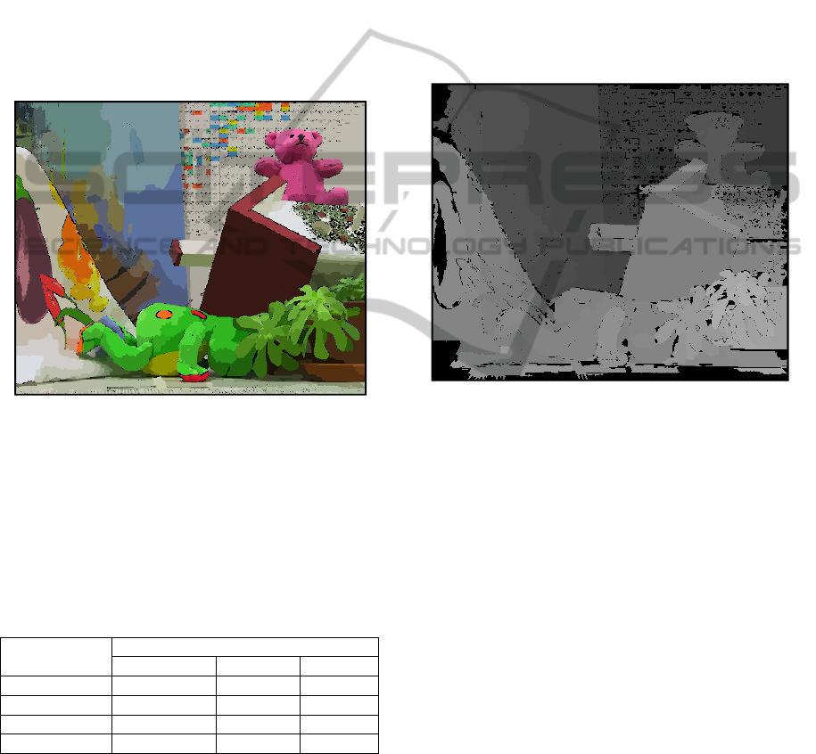
An example of result obtained with CSC method
when applied to Teddy left image is shown in Figure
6. The only parameter in this method is a threshold,
fixed on 24 for all our experiments.
3 RESULTS
We applied the suggested approach to the same 4
(four) images studied in Table 1. Those results were
evaluated through the same criteria as in Table 1.
Figure 7 shows the resulting image for the Teddy
image, while Table 3 contains the evaluation results
for the experiment.
Figure 6: Result of CSC method applied to Teddy image.
This approach has improved the original’s
method score on (Middlebury, 2011). One of the
main contributions for that accomplishment is the
edge preserving of the objects on images. That
enhance on edges is derived directly from the image
segmentation algorithm.
Table 3: Proposed method evaluation (Closer to 0.0 best.
Closer to 100.0 worst). Threshold = 2.
Image
Evaluation
nonocc all disc
Tsukuba 4.17 4.68 15.3
Venus 4.13 4.54 12.8
Teddy 14.1 17.6 23.9
Cones 8.44 15.4 15.7
On the other hand. Even after getting quite
higher scores, there are still some problems to be
solved. As shown in Figure 7, there are several small
regions in black color. Those regions are called
unsolved regions and that is either because of small
faults on segmentation algorithm (black dots on
Figure 6) or because of an inexistence of intersection
between a sparse correspondence (Figure 5) and an
image segment (Figure 6).
4 CONCLUSIONS
The proposed method is able to improve the LM’s
score on (Scharstein and Szeliski, 2002) evaluation’s
method. That is significant improvement, since it
went from a very low score to a higher one. That
improvement was also enough to get this method
ahead of at least 10 other correspondence
approaches that are ranked at (Middlebury, 2011).
Figure 7: Result of the proposed method when applied to
Teddy image.
We also have several improvements to study. For
example: the occurrence of inclination of some
objects along Z axis. Small inclinations would result
in smaller errors, while big inclinations would end in
bigger errors. Other points we are studying are: 1)
the development of a color-based indexation, instead
of intensity-based (for better indexing results); and
2) fixing the unsolved regions, detailed in the
previous section.
REFERENCES
Klaus, A., Sormann, M. and Karner, K. 2006. Segment-
based stereo matching using belief propagation and a
self-adapting dissimilarity measure. ICPR '06
Proceedings of the 18th International Conference on
Pattern Recognition.
Murray, D., Little, J. J., 2000. Using Real-Time Stereo
Vision for Mobile Robot Navigation. In Autonomous
Robots, Volume 8, Number 2. SpringerLink.
Oliveira, M. A. F. de, Wazlavick, R. S., 2005. Linear
Complexity Stereo Matching Based on Region
LINEAR COMPLEXITY STEREO CORRESPONDENCE - From Interpolation to Segment-based Approach
311

Indexing. In Proceedings of the XVIII Brazilian
Symposium on Computer Graphics and Image
Processing - SIBGRAPI’05, IEEE Computer Society.
Natal.
Rehrmann, V., Priese, L. 1997. Fast and Robust
Segmentation of Natural Color Scenes. In Proceedings
of the 3 rd Asian Conference on Computer Vision.
Springer Verlag, pages 598-606.
Scharstein , D., Szeliski, R. 2002. A taxonomy and
evaluation of dense two-frame stereo correspondence
algorithms. International Journal of Computer Vision,
47:7–42.
Scharstein , D., Szeliski, R. 2003. High-accuracy stereo
depth maps using structured light. In IEEE Computer
Society Conference on Computer Vision and Pattern
Recognition, volume 1, pages 195–202.
Middlebury Stereo Evaluation, 2011. Available at
http://vision.middlebury.edu/stereo/eval/.
ICINCO 2011 - 8th International Conference on Informatics in Control, Automation and Robotics
312
