ADAPTIVE CONTINUOUS HIERARCHICAL MODEL-BASED
DECISION MAKING
For Process Modelling with Realistic Requirements
Kamil Dedecius
Institute of Information Theory and Automation, Academy of Sciences of the Czech Republic
Pod Vod´arenskou vˇeˇz´ı 4, 182 08 Prague, Czech Republic
Pavel Ettler
COMPUREG Plzeˇn, s.r.o., N´adraˇzn´ı 18, 306 34 Plzeˇn, Czech Republic
Keywords:
Bayesian modelling, Hierarchical model, Parameter estimation, Cold strip rolling, Rolling mills.
Abstract:
Industrial model-based control often relies on parametric models. However, for certain operational conditions
either the precise underlying physical model is not available or the lack of relevant or reliable data prevents its
use. A popular approach is to employ the black box or grey box models, releasing the theoretical rigor. This
leads to several candidate models being at disposal, from which the (often subjectively) prominent one is se-
lected. However, in the presence of model uncertainty, we propose to benefit from a subset of credible models.
The idea behind the multimodelling approach is closely related to hierarchical modelling methodology. By
using several modelling levels, it is possible to achieve relatively high quality and robust solution, providing a
way around typical constraints in industrial applications.
1 INTRODUCTION
Industrial model-based control or prediction is con-
nected with several practical but often contradictory
requirements:
– The model should respect physical relations of the
process yet be simple enough;
– The model should approximate process behaviour
in all possible working conditions;
– Imperfection of measured data feeding the model
should not deteriorate control or prediction qual-
ity.
Possible solution of the first two above-mentioned is-
sues consists in switching amongseveral proven mod-
els according to actual working conditions. The third
problem is much more difficult to be solved in princi-
ple. The data driven (black box) models could seem
to be most appropriate but they almost always con-
tradict the first two requirements. See, e.g., (Bohlin,
1991) for remarks on black and grey box modelling.
On-line mixing of several proven process mod-
els – which can be considered as continuous decision
making – turns out to be a solid compromise solution
of all three requirements, at least for the process of
cold strip rolling from which comes the motivation
for this research (Ettler and Andr´ysek, 2007).
The presented method of model mixing is closely
related to dynamic model averaging (Raftery et al.,
2010). However, two additional requirements stimu-
lated the need for a specific solution:
– Sum of weights corresponding to particular mod-
els is required to be always equal to one;
– An offset term should be continuously estimated
to eliminate any residual discrepancy, whatever it
comes from.
While the first restriction can be easily justified
from the probabilistic point of view, insistence on the
second requirement comes purely from practical ex-
perience, although the existence of the offset might
theoretically be superfluous. Presented solution at-
tempts to reconcile both requirements.
The method is developed in the Bayesian frame-
work, treating the unknown parameters as random
variables. Each model is represented by a condi-
tional probability density function (pdf) of the mod-
elled variable, given a set of features and parameters.
The layout of the paper is as follows: Section 2 de-
scribes the structure of the multimodel and its levels;
in Section 3 we derive a particular case of the model.
284
Dedecius K. and Ettler P..
ADAPTIVE CONTINUOUS HIERARCHICAL MODEL-BASED DECISION MAKING - For Process Modelling with Realistic Requirements.
DOI: 10.5220/0003533402840289
In Proceedings of the 8th International Conference on Informatics in Control, Automation and Robotics (ICINCO-2011), pages 284-289
ISBN: 978-989-8425-74-4
Copyright
c
 2011 SCITEPRESS (Science and Technology Publications, Lda.)

Section 4 contains an example of application. Finally,
Section 5 concludes the achievements.
2 HIERARCHICAL MODELLING
CONCEPT
Assume, that there is a stochastic system observed at
discrete time instants k = 1, 2, . . . , which is to be mod-
elled. The statistical framework employs, among oth-
ers, parametric models, expressing the dependence of
the output variable of interest y
k
on a nonempty or-
dered set of observed data
D (k) = {d
κ
}
κ=0,...,k
, d
κ
∈ R
n
.
d
0
is the prior knowledge represented, for instance,
by an expert information or a noninformative distri-
bution. The task is to predict the future output y
k+1
,
e.g., for control.
Often there is a whole set of available models,
mainly those based on underlying physical principles
of the process. However, since in many applications
either the precise physical model is not available or
the lack of reliable data prevents its use, the user em-
ploys black box or grey box models. Then, either the
(subjectively) best model or models are selected and
switched or, alternatively, a rich-structure model be-
ing a union of several candidate models is built. De-
spite the potential applicability of the latter case, the
over-parametrization in combination with unreliable
measurements and their traffic delays is expected to
be fatal.
Our method provides a way around most of disad-
vantages of the mentioned approaches. We propose a
hierarchical model composed of three levels:
Low-level Models comprise arbitrary count of plau-
sible parametric models like the regressive and the
space-state ones. They are independent of each
other, but their aims are identical – modelling of
the same quantity of interest.
Averaging Model is intended for merging the infor-
mation from the low-level models. The resulting
mixture of predictive pdfs of low-level models,
weighted by their evidences, is used to evaluate
the predictions.
High-level Model – since industry has several spe-
cific requirements related, e.g., to stable control,
we add a high-level model. It provides stabiliza-
tion of the prediction process. However, the goal
of this level can differ from case to case according
to specific needs of the field of application being
addressed.
The ensuing sections describe these levels in some de-
tail.
2.1 Low-level Models
The low-level modelsexpress the relationbetween the
actual system output y
k
and the given data D (k) by a
pdf
f(y
k
|D (k− 1), Θ), (1)
where Θ denotes a multivariate finite model parame-
ter which, underthe Bayesian treatment, is considered
to be a random variable obeying pdf
g(Θ|D (k− 1)). (2)
If this pdf is properly chosen from a class conjugate
to the model (1), the Bayes’ theorem yields a poste-
rior pdf of the same type (Bernardo and Smith, 2001).
Then, the rule for recursive incorporationof new mea-
surements into the parameter pdf reads
g(Θ|D (k)) =
f(y
k
|D (k− 1), Θ)g(Θ|D (k− 1))
I
k
,
(3)
where
I
k
=
Z
f(y
k
|D (k− 1), Θ)g(Θ|D (k− 1))dΘ (4)
= f(y
k
|D (k− 1)) (5)
is a normalizing term. It assures unity of the resulting
pdf and it is a suitable measure of model’s fit, often
called evidence. The equality of (4) and (5) follows
from the Chapman-Kolmogorov equation (Karush,
1961). Furthermore, this equation also yields the pre-
dictive pdf f (y
k+1
|D (k)) providing the Bayesian pre-
diction, formally
f(y
k+1
|D (k)) =
Z
f(y
k+1
|D (k), Θ)g(Θ|D (k))dΘ
=
I
k+1
I
k
. (6)
The last equality follows from the recursive property
of the Bayesian updating (3).
Although the described methodology is important
per se, it strongly relies on invariance of Θ. However,
this assumption is often violated in practical situations
and the evolution ofΘ must be appropriatelyreflected
by an additional time update according to model
g(Θ
k+1
|Θ
k
, D (k)). (7)
Generally, we can distinguish two significant cases:
(i) The evolution model (7) is known a priori. Then,
Θ is called the state variable and, under certain
conditions, the modelling turns into the famous
Kalman filter (Peterka, 1981).
ADAPTIVE CONTINUOUS HIERARCHICAL MODEL-BASED DECISION MAKING - For Process Modelling with
Realistic Requirements
285

(ii) The model (7) is unknown, but slow variability
of Θ is assumed. This case is usually solved ei-
ther by finite window methods or by forgetting.
The latter heuristically circumvents the model ig-
norance by discounting of potentially outdated in-
formation from the parameter pdf. Formally, it
introduces a forgetting operator F modifying the
posterior pdf,
g(Θ
k+1
|D (k)) = F [g(Θ
k
|D (k))] .
The class of available forgetting methods com-
prises, e.g., exponential forgetting (Peterka,
1981), directional forgetting (Kulhav´y and K´arn´y,
1984), partial forgetting (Dedecius, 2010) and
others.
Since the issue of parameter variability is behind the
scope of the paper, we can stick with unsubscripted Θ
without a loss of generality.
2.2 Averaging Model
Assume that there is a nonempty finite set of differ-
ent low-level models M = {M
(1)
, . . . , M
(S)
}, S ∈ N,
which are considered as candidates to represent the
system under study. Formally, we have
M
(s)
: f(y
k
|D (k− 1), Θ
(s)
, M
(s)
), s = 1, . . . , S, (8)
which directly coincide with (1). These models are
independently evaluated in accordance with Section
2.1. Their probabilitiesare expressed by a distribution
h(M |D (k)) ≡ h(M
(1)
, . . . , M
(S)
|D (k)). (9)
The averaging model evaluates this distribution with
respect to evidences (5) of low-level models (8) on
base of marginal pdfs, namely
h(M
(s)
|D (k)) ∝ h(M
(s)
|D (k− 1)) I
(s)
k
, (10)
where ∝ denotes equality up to a normalizing factor.
The prior distribution h(M
(s)
|D (0)) can be chosen ei-
ther on base of expert information or as noninforma-
tive pdf with equal marginals.
The predictive pdf of the system output given the
set of data D (k) and the set of models M is repre-
sented by a mixture
f(y
k+1
|D (k), M )
=
K
∑
k=1
f(y
k+1
|D (k), M
(s)
)h(M
(s)
|D (k)). (11)
The point estimate of y
k+1
provides the mixture (11)
in the form of a convexcombination of weightedpoint
estimates E
h
y
k+1
|D (k), M
(s)
i
. It coincides with the
method of Dynamic model averaging (Raftery et al.,
2010).
2.3 High-level Model
The purposeof the high-level model is stabilization of
the prediction, particularly for its further use in con-
trol. Inclusion of the third modelling level is justified
by practical experience with averaging models which,
in contrast to theoretical assumptions, may provide
biased results. The most basic high-level model can
be represented by a pdf
f(˜y
k+1
|D (k), ˆy
k+1
,
˜
Θ), (12)
where ˜y
k+1
is recursively modelled given the features
– point estimates of ˆy
k+1
obtained from the averag-
ing model. The high-level model is parametrized by
a multivariate parameter
˜
Θ. The point estimate ˜y
k+1
is the output of the hierarchical model. This provides
the solution to the task stated in Section 2.
3 ELABORATION FOR
INDUSTRIAL APPLICATION
This section elaborates the method for a particular but
important case of normal regressive models at the low
level. The generalization for another cases, e.g., the
state-space models like the Kalman filter and its vari-
ants is straightforward and the averaging model re-
mains unchanged. For the sake of convenience, the
evolution of parameters will not be discussed.
3.1 Low-level Models
We consider a normal linear regressive model with a
regressor ψ
k
∈ R
n
and a vector of regression coeffi-
cients θ of the same dimension, i.e.
y
k
= ψ
′
k
θ + e
k
, (13)
where e
k
∼ N (0, σ
2
) is the additive normal white
noise. The Bayesian framework relates it with (1)
through pdf
f(y
k
|D (k− 1), Θ) ∼ N (ψ
′
k
θ, σ
2
), (14)
where
Θ ≡ {θ, σ
2
}.
An appropriate distribution conjugate to the model
(14) is of the normal inverse-gamma type (Murphy,
2007),
g(Θ|D (k)) ∼ N iΓ(V
k
, ν
k
), (15)
where V
k
∈ R
N×N
is an extended information matrix,
i.e., a symmetric positive definite square matrix of di-
mension N = n + 1, and ν
k
∈ R
+
is a number of de-
grees of freedom. The Bayes’ theorem (3) updates
these two statistics by new data as follows:
ICINCO 2011 - 8th International Conference on Informatics in Control, Automation and Robotics
286

V
k
= V
k−1
+

y
k
ψ
k

y
k
ψ
k

′
ν
k
= ν
k−1
+ 1.
It may be proved(Peterka, 1981) thatthe estimator
of θ = (θ
1
, . . . , θ
n
)
′
is
ˆ
θ =



ˆ
θ
1
.
.
.
ˆ
θ
n



=



V
21
.
.
.
V
N1



′



V
22
. . . V
2N
.
.
.
.
.
.
.
.
.
V
N2
. . . V
NN



−1
.
This relation is equivalent to the recursive least
squares (Peterka, 1981) and it provides the estimates
for prediction with (13). The normalizing integral I
k
is nontrivial, it can be found, e.g., in (Peterka, 1981;
K´arn´y, 2006).
Since the information matrices are often ill-
conditioned and their inversions can lead to signif-
icant numerical issues, it is reasonable to evaluate
calculations on factorized forms, e.g., the Cholesky,
UDU’ or SVD ones.
3.2 Averaging Model
The averaging model introduced in Section 2.2 is re-
sponsible for merging the informationfrom the under-
laying low-level models. For the sake of better read-
ability, let us denote
α
(s)
k
≡ h(M
(s)
|D (k)).
The point prediction of the output at this modelling
level follows from (11), hence it reads
ˆy
k+1
=
K
∑
k=1
E
h
y
t+1
|D (k), M
(s)
i
α
(s)
k
. (16)
From the statistical viewpoint, two cases can occur.
The latter one is a generalization of the former one;
both are described below.
3.2.1 Two Low-level Models
Assume that we have two models M
(1)
and M
(2)
with
real nonnegative scalar statistics a
(1)
and a
(2)
. We
want these models to have probabilities α for M
(1)
and 1 − α for M
(2)
. Then, the distribution of mod-
els can be viewed as the beta distribution (Gupta and
Nadarajah, 2004) with pdf
f(α|a
(1)
, a
(2)
) =
Γ(a
(1)
+ a
(2)
)
Γ(a
(1)
)Γ(a
(2)
)
α
a−1
(1− α)
a
(2)
−1
where Γ stands for the gamma function. The point
estimate of the mean value and the variance are
ˆ
α = E
h
α|a
(1)
, a
(2)
i
=
a
(1)
a
(1)
+ a
(2)
, (17)
var(α) =
a
(1)
a
(2)
(a
(1)
+ a
(2)
)
2
(a
(1)
+ a
(2)
+ 1)
.
The rule for update of statistics a
(1)
and a
(2)
is as
follows:
a
(1)
k
= α
k−1
I
(1)
k
a
(2)
k
= (1 − α
k−1
)I
(2)
k
(18)
3.2.2 Multiple Low-level Models
The distribution of probabilities of multiple models
M
(1)
, . . . , M
(S)
can be derived as a generalization of
the beta pdf. Let a = (a
(1)
, . . . , a
(S)
) be a vector of
nonnegative real statistics. Furthermore, let us intro-
duce independent identically distributed (i.i.d.) ran-
dom variables W
(s)
∼ Γ(a
(s)
, 1), s = 1, . . . , S and set
W = (W
(1)
, . . . , W
(S)
), T =
S
∑
s=1
W
(s)
,
α = (α
(1)
, . . . , α
(S)
) where α
(s)
=
W
(s)
T
. (19)
Obviously, (19) imposes constraints α
(s)
∈ [0, 1] and
∑
α
(s)
= 1. Since the pdf of a gamma distribution for
W
(s)
is
f(W
(s)
|a
(s)
, 1) =
1
Γ(a
(s)
h
W
(s)
i
a
(s)
−1
e
−W
(s)
,
the pdf for the multivariate W with i.i.d. elements has
the form
f(W |a, 1) =
S
∏
s=1
1
Γ(a
(s)
)
h
W
(s)
i
a
(s)
−1
e
−W
(s)
.
Since α’s should sum to unity, we need only (S−
1)-variate vector α = (α
(1)
, . . . , α
(S−1)
). The change
of variables theorem (Rudin, 2006) provides a way to
interchange of W
(s)
and α
(s)
,
f(α|·) = f
W
(α|·)detJ
W →α
.
Here, J
W →α
denotes the Jacobian matrix contain-
ing partial derivatives of the projection and f
W
(α|·)
is originally a function f(W |a, 1) with α substi-
tuted for W . Since W
(s)
= Tα
(s)
is bijective for
s = 1, . . . , S− 1 andW
(S)
= T(1−α
(1)
−. . . − α
(S−1)
),
the necessary condition is fulfilled and the theorem
may be used. The determinant of the Jacobian
J
W →α
= det

∂W
∂α
,
∂W
∂T

= T
S−1
provides
f(α, T) = T
A−1
e
−T
S
∏
s=1
1
Γ(a
(s)
)
h
α
(s)
i
a
(s)
−1
,
ADAPTIVE CONTINUOUS HIERARCHICAL MODEL-BASED DECISION MAKING - For Process Modelling with
Realistic Requirements
287

where A =
∑
k
a
(s)
. Integrating T out with the rule
Z
T
A−1
e
−T
dT = Γ(A)
leads to the pdf of α as follows:
f(α|a) =
Γ(A)
∏
S
s=1
Γ(a
(s)
)
S
∏
s=1
h
α
(s)
i
a
(s)
−1
This pdf is a variant of the Dirichlet distribution
(Geiger and Heckerman, 1997), with nonnegative real
statistics a
(s)
. Since the marginal distributions are of
beta type B(a
(s)
, A−a
(s)
), the estimator of kth element
of α is
E
h
α
(s)
i
=
ˆ
α
(s)
=
a
(s)
A
=
a
(s)
∑
S
s=1
a
(s)
and its variance is
var(α
(s)
) = α
(s)
A− α
(s)
A
2
(A+ 1)
.
The rule updating statistics a
(s)
is a straightfor-
ward generalization of (18)
a
(s)
k
= α
(s)
k−1
I
(s)
k
.
3.3 High-level model
The high-level model discussed in Section 2.3 stabi-
lizes the prediction according to specific needs of the
application field of interest. In our case, we use a nor-
mal regressive model equivalent to (14) with a regres-
sor being composed of the averaging model output
ˆy
k+1
(16) and an offset term,
ψ
k
= ( ˆy
k+1
, 1)
′


D (k), M .
Its evaluation, i.e., parameter estimation and output
prediction, follows from Section 3.1.
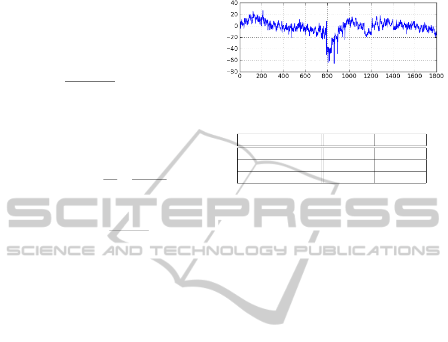
4 REAL DATA EXAMPLE
Let us demonstrate the presented method on a simpli-
fied example. Used data come from a four-high cold
rolling mill and the aim consists in reliable instanta-
neous prediction of the output strip thickness devia-
tion (denoted h
2
), measurable only with a significant
time delay. The true evolution of the modelled out-
put strip thickness deviation (h
2
) is depicted in Fig. 1.
Apparently, we can experience modelling difficulties
around k ≈ 800, where the data abruptly changed.
Three simple low-level models were chosen to
Figure 1: Evolution of the output strip thickness deviation
h
2
[µm].
Table 1: Statistics of the prediction error.
Statistics \ Model averaging high-level
mean error 0.20 0.04
standard deviation 6.42 5.78
median 0.27 -0.06
approximate relations among selected process vari-
ables. They are characterized by the following regres-
sor structures:
M
(1)
: ψ = (v
r
, h
1
v
r
, 1)
′
,
M
(2)
: ψ = (h
1
, z, 1)
′
,
M
(3)
: ψ = (h
1
, z, v
r
, 1)
′
,
where v
r
denotes the ratio of the input and output strip
speeds, h
1
is the deviation of the input strip thick-
ness from its nominal value and z stands for the so
called uncompensated rolling gap. See (Ettler and
Andr´ysek, 2007) for details.
The initial setting was as follows: the low-
level models started with noninformative priornormal
inverse-gamma distributions (15). Forgetting factor
of the applied exponential forgetting (Peterka, 1981)
was set to 0.99. The averaging model started with
uniformlydistributed prior statistics a
(s)
0
, s = {1, 2, 3}.
The high-level model with the structure given in Sec-
tion 3.3 started with a noninformative prior pdf with
similar initial statistics as the low-level models. For-
getting factor was set to 0.98 in this case.
The evolution of probabilities of the averaged
models M
(s)
, s = {1, 2, 3} is depicted in Fig. 3. The
evolution of prediction error for h
2
is depicted in Fig.
2. Obviously, the announcedabrupt change in the data
course led to higher prediction errors. Statistics of the
prediction error stated in Tab. 1 demonstrate the role
of the high-level modelling.
5 CONCLUSIONS
A method of multilevel modelling was proposed to
improve instantaneous prediction of a key variable in
the process of cold strip rolling. The resulting hier-
archical model consist of three modelling levels – the
ICINCO 2011 - 8th International Conference on Informatics in Control, Automation and Robotics
288

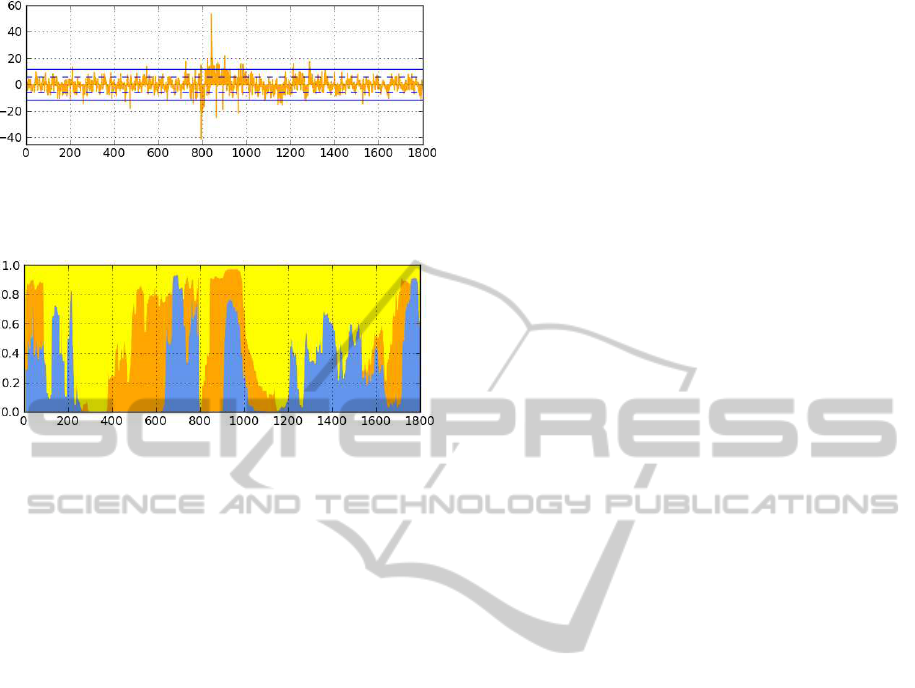
Figure 2: Absolute prediction error [µm]: dashed and solid
line denote the distance of one and two standard deviations,
respectively.
Figure 3: Evolution of probabilities of models: M
(1)
(blue),
M
(2)
(orange) and M
(3)
(yellow).
low-level models, i.e., from the statistical viewpoint
usual parametric models, the averaging model merg-
ing their results and the high-level model, reflecting
specific needs of the application field. Each mod-
elling level is treated in the Bayesian framework, i.e.,
both the models and their parameters are represented
by conditional distributions. Current state of the re-
search was demonstrated on a simple example utiliz-
ing real industrial data. Extensive tests will be accom-
plished to refine the method and prepare algorithms
for a true on-line industrial application.
ACKNOWLEDGEMENTS
This research was supported by project M
ˇ
SMT
7D09008 (ProBaSensor) and project 1M0572 (DAR).
REFERENCES
Bernardo, J. and Smith, A. (2001). Bayesian Theory. Mea-
surement Science and Technology, 12:221.
Bohlin, T. (1991). Interactive System Identification:
Prospects and Pitfalls. Springer-Verlag, Berlin, Hei-
delberg, New York.
Dedecius, K. (2010). Partial Forgetting in Bayesian Es-
timation. PhD thesis, Czech Technical University in
Prague.
Ettler, P. and Andr´ysek, J. (2007). Mixing Models to Im-
prove Gauge Prediction for Cold Rolling Mills. In
Proceedings of the 12th IFAC Symposium on Automa-
tion in Mining, Mineral and Metal Processing, Que-
bec, Canada.
Geiger, D. and Heckerman, D. (1997). A Characterization
of the Dirichlet Distribution Through Global and Lo-
cal Parameter Independence. The Annals of Statistics,
25(3):1344–1369.
Gupta, A. and Nadarajah, S. (2004). Handbook of Beta Dis-
tribution and its Applications. CRC.
K´arn´y, M. (2006). Optimized Bayesian Dynamic Advising:
Theory and Algorithms. Springer-Verlag New York
Inc.
Karush, J. (1961). On the Chapman-Kolmogorov Equation.
The Annals of Mathematical Statistics, 32(4):1333–
1337.
Kulhav´y, R. and K´arn´y, M. (1984). Tracking of Slowly
Varying Parameters by Directional Forgetting. In 9th
IFAC World Congress, Budapest, Hungary.
Murphy, K. (2007). Conjugate Bayesian Analysis of the
Gaussian Distribution.
Peterka, V. (1981). Bayesian Approach to System Iden-
tification In P. Eykhoff (Ed.) Trends and Progress in
System Identification.
Raftery, A., K´arn´y, M., and Ettler, P. (2010). Online Pre-
diction Under Model Uncertainty via Dynamic Model
Averaging: Application to a Cold Rolling Mill. Tech-
nometrics: a journal of statistics for the physical,
chemical, and engineering sciences, 52(1):52.
Rudin, W. (2006). Real and complex analysis. Tata
McGraw-Hill.
ADAPTIVE CONTINUOUS HIERARCHICAL MODEL-BASED DECISION MAKING - For Process Modelling with
Realistic Requirements
289