DESIGN APPROACH OF DISTRIBUTED SYSTEMS FOR THE
CONTROL OF INDUSTRIAL PROCESS
D. Boudebous, J. Boukachour, S. Benmansour and N. Smata
Laboratory CERENE, ISEL quai Frissard BP 1137 76603, Le Havre cedex, France
Keywords: Control system, Industrial processes, Physical processes, Temporal dependence, Petri nets.
Abstract: This article describes a methodological approach to the design of distributed systems for the control of
industrial process. The designer tackles the problem by specifying the behaviour of the process rather than
by specifying a solution. In this way he defines the “what to control”. This specification can then be
converted not only into a Petri net to allow the checking of certain properties of the described behaviour, but
also into a logical network of communicating modules which defines the logical structure of the process
control system. In both cases, the rules of conversion are direct and simple.
1 INTRODUCTION
In various fields of application, the constraints that
computer systems have to take into account
increasingly force their design as distributed
systems. Also, at various stages of design, the need
to take into account the expression of the
distribution (Chen and Yeh, 1983), (Krause and all,
2009), (Lamport, 1983), as well as the expression of
parallelism, soon makes itself felt. However, in the
face of the complexity of the problems to be
resolved, the effective utility of such linguistic tools
remains largely dependent on methodological
analysis and design guides, which allow us to move
from the wording of the problem to a choice of
solutions.
In this article we present a methodological
approach to the design of distributed systems for the
control of production systems, which can guide the
designer from the initial specification of a problem
right up to the implementation of his solution on an
execution structure. In this approach we identify
three stages:
• the logical construction of the control system in
terms of communicating modules;
• the detailed design of the modules and their
programming;
• the definition of a system execution structure.
These three stages allow the gradual construction, by
levels of abstraction, of a solution which is, as far as
possible, independent of the physical network of the
sites. In this article we tackle the first stage by
presenting an approach which uses a coherent
combination of guides and tools, to facilitate the
construction, specification and correction of the
logical structure of industrial process design systems
in terms of communicating modules (Kramer and
all, 1989), (Kramer and all, 1983). This approach is
based essentially on a problem-oriented approach. In
comparison with other methods, the designer does
not approach the logical structuring of his control
system by asking himself at the outset “how to
control” his industrial process. Instead he
approaches the problem by first asking himself
“what to control”. Rather than specify the control
system, he specifies the behaviour of the industrial
process by identifying the existing physical
processes and their temporal dependences. It is this
specification which constitutes the terms of the
problem to be resolved and which is then used to
deduce the logical structuring of his control system.
He considers for this that the modular entities of his
control system are merely abstract views of the
physical processes of his industrial process and that
the temporal relationships which interlink these
physical processes specify the inter-modular
behaviour of the control system. It is during this
phase dedicated to the analysis of “what to control”
rather than “how to control” that the designer is best
placed to make good choices which guarantee the
quality of the functional breakdown (clarity,
efficacy, robustness, maintainability and reusability)
and which take into account the constraints of the
157
Boudebous D., Boukachour J., Benmansour S. and Smata N..
DESIGN APPROACH OF DISTRIBUTED SYSTEMS FOR THE CONTROL OF INDUSTRIAL PROCESS.
DOI: 10.5220/0003438801570164
In Proceedings of the 13th International Conference on Enterprise Information Systems (ICEIS-2011), pages 157-164
ISBN: 978-989-8425-55-3
Copyright
c
 2011 SCITEPRESS (Science and Technology Publications, Lda.)

problem posed (flexibility in the distribution of the
control system in different sites, parallelism and
safety). It is also the optimum moment to discuss
his choices with the user.
In this article we deal with the modelling of the
behaviour of the processes. We present the
formalisms (textual and graphic) which enable the
specification of this behaviour by following a
top-down or a bottom-up approach. This
specification can then be directly converted into a
Petri net (Brams, 1983) (Cao and all, 2003)
(Drzymalski and Odrey, 2008) so that the
behavioural properties of the modelled process can
be checked. We will then demonstrate that it is
equally possible, through direct and simple
conversion, to pass from this specification of the
system behaviour to the logical construction of the
control system in terms of communicating modules.
Finally we will illustrate our argument with an
example.
2 THE INDUSTRIAL PROCESS
DESCRIPTION MODEL
An industrial system is defined by a set of entities
(trucks, robots, atmospheric environment, …) whose
attributes are likely to evolve with time, and also by
a set of physical processes. At any given moment
the physical state of the process is determined by the
attributes of its entities. This physical state could
correspond to a state of normal functioning or to a
state of breakdown. The role of the individual
physical processes is to enable the industrial system
to evolve from one state to another, by carrying out a
particular physical activity in a determined time.
The process model is represented by <P, Q, C>
where:
• P represents the set of physical processes p
i
,
• Q the set of its physical states q
i
,
• and C its behaviour.
If a
ij
is the jth activity carried out by the physical
process p
i
, then t(a
ij
) denotes the start date of this
activity and t’(a
ij
) its finish date.
The history of a physical process p
i
at any given
moment is defined by the chronological order of the
activities carried out since the start of the system.
This order is expressed as h
i
= (a
i0
, a
i1
, ....., a
in
)
where t’(a
ij
)≤ t(a
ij+1
). The behaviour of a process
defines a partial order among the elements of the
orders h
i
of the set of the physical processes p
i
. This
ordering is determined by four types of temporal
dependence which interlink the physical processes.
These are: causal precedence, coupling, temporal
precedence and independence which are defined in
Sections 2.1, 2.2, 2.3 and 2.4.
To specify the behaviour of a process we present
two formalisms. The first allows us to specify
independently for each physical process p
i
of the
process, all its direct temporal dependences, with the
help of temporal relationship operators (
″→″ for
causal precedence,
″⇒″ for coupling, and ″ --> ″ for
temporal precedence) and physical process
composition operators
″ * ″ (and), ″ + ″ (or) and ″⊕″
(xor).
The second formalism permits the specification
of the temporal dependences of the physical
processes in a graphical form close to that of Petri
nets (Dong and all, 2001) (Kara and all, 2009). In
this formalism the places are labelled and retain their
habitual representation and meaning. We call E the
set of labels e
i
associated with these places. We can
associate each of these labels with a specific
physical state defined in Q. We call R: E*Q the
relationship which joins a physical state q
j
to each
place e
i
. The transitions represented by rectangles
correspond to the physical processes p
i
of the
system. These transitions are not necessarily atomic:
new rules, according to the temporal dependences of
the process concerned, define the conditions of
activation and the effect of an activation on the input
and output places of a transition. The type of
dependence is determined by the type of arcs which
link the places and the transitions between them
(″→″ for causal precedence, ″•⇒″ and ″⇒•″ for
coupling, and ″-->″ for temporal precedence).
A marking M: is a function from P*E → Ν (where
Ν is the set of positive integers).
M(p
i
,e
j
) denotes the number of tokens in the place e
j
before activation of the physical process p
i
, and
M’(p
i
,e
j
) denotes the number of tokens in the place e
j
after activation of the physical process p
i
M(-,e
j
) denotes the initial state of the place e
j
.
The two formalisms used are equivalent. In
comparison with Petri nets, this type of formalism
permits a more concise expression which is thus
easier to read and to write. It can be converted into a
Petri net to enable the formal checking of the
properties of the described behaviour. In the
following paragraphs we will deal more precisely
with the definition of the different temporal
dependences and their specification in the two
formalisms, before addressing, in Sections 3 and 4,
the approach to modelling and to checking the
behavioural properties of a process.
ICEIS 2011 - 13th International Conference on Enterprise Information Systems
158

2.1 Causal Precedence
Given two physical processes p
1
and p
2
of an
industrial system, if h
1
= (a
10
, a
11
, ...., a
1n
, ...) and
h
2
= (a
20
, a
21
, ...., a
2n
, ...) respectively represent their
histories, we will say that p
1
precedes p
2
and we
write p
1
Ù p
2
if at any given moment for each
couple (a
1k
, a
2k
) we have t’(a
1k
) ≤ t’(a
2k
), if this
condition is not met we write ⎤( p
1
Ù p
2
).
p
1
→ p
2
if and only if
(1) p
1
Ù p
2
(2) there exists no p
i
such that p
1
Ù p
i
et p
i
Ù p
2
(3) there exists no p
i
≠ p
1
such that p
i
Ùp
2
et
⎤( p
i
Ù p
1
)
(4) there exists no p
j
≠ p
2
such that p
1
Ù p
j
et
⎤( p
2
Ù p
j
)
We will say that p
1
is the immediate predecessor
of p
2
and that p
2
is the immediate successor of p
1
.
We can deduce from this on the one hand that p
2
can
only start an activity if and only if p
1
finishes an
activity and on the other hand that each completion
of activity p
1
can lead only to the start of an activity
by p
2
. These definitions relate to the definitions of
precedence and causal precedence presented for the
events in (Baker and Hewitt, 1997). In a relationship
of causal precedence we can describe a physical
process as having several immediate successors or
several immediate predecessors. For this we use the
physical process composition operators ″*″ , ″+″
and ″⊕″. The basic notation of such temporal
relationships is defined in Table 1. These basic
relationships can be combined to express more
complex temporal relationships, in which the usual
rules of parenthesis allow the definition of priorities
among the composition operators.
2.2 Coupling
Given two physical processes p
1
and p
2
of an
industrial system, if h
1
= (a
10
, a
11
, ...., a
1n
, ...) and
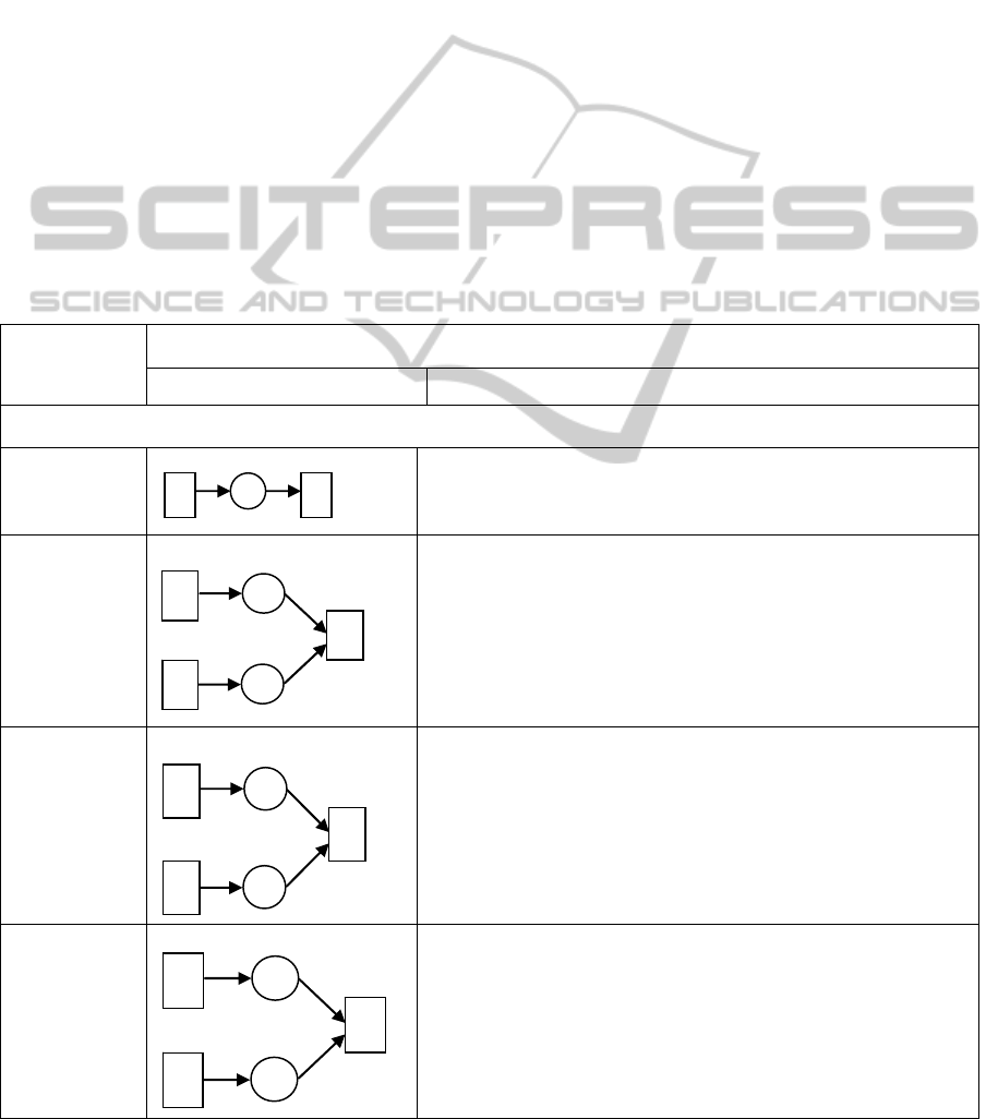
Table 1: Basic notation of causal precedence relationships.
Textual Form Graphical Form
Representation Rules of progress of the token
Designation of immediate predecessors
p
1
→ p
2
Before activation of p
2
: M(p
2
,e
1
)>0
After activation of p
2
: M’(p
2
,e
1
)=M(p
2
,e
1
)-1
p
1
+ p
2
→ p
3
Before activation of p
3
: M(p
3
,e
1
)>0 or M(p
3
,e
2
)>0
After activation of p
3
: M’(p
3
,e
1
)=if M(p
3
,e
1
)>0 then
M(p
3
,e
1
)-1 or M(p
3
,e
1
) else M(p
3
,e
1
) and
M’(p
3
,e
2
)= if M(p
3
,e
2
) > 0 then M(p
3
,e
2
)-1 or M(p
3
,e
2
)
else
M(p
3
,e
2
) and M’(p
3
,e
1
) + M’(p
3
,e
2
)= M(p
3
,e
1
)+ M(p
3
,e
2
) – 1
p
1
* p
2
→ p
3
Before activation of p
3
: M(p
3
,e
1
)>0 and M(p
3
,e
2
)>0
After activation of p
3
: M’(p
3
,e
1
) = M(p
3
,e
1
) - 1 and
M’(p
3
,e
2
) = M(p
3
,e
2
) - 1
p
1
⊕p
2
→ p
3
Before activation of p
3
: M(p
3
,e
1
)>0 and M(p
3
,e
2
)=0 or
M(p
3
,e
1
)=0 and M(p
3
,e
2
)>0
After activation of p
3
: M’(p
3
,e
1
) = if M(p
3
,e
1
)>0 then
M(p
3
,e
1
)-1 else M(p
3
,e
1
) and
M’(p
3
,e
2
) = if M(p
3
,e
2
)>0 then M(p
3
,e
2
) -1 else M(p
3
,e
2
)
e
1
p
1
p
2

e
1
p
2
p
1
p
3
*
e
2

⊕
p
2
p
1
p
3
e
2
e
1

e
1
p
2
p
1
p
3
+
e
2
DESIGN APPROACH OF DISTRIBUTED SYSTEMS FOR THE CONTROL OF INDUSTRIAL PROCESS
159

h
2
= (a
20
, a
21
, …., a
2n
, ...) represent their respective
histories, we will say that p
2
is coupled to p
1
for its
start if at any given moment, whatever a
21
denotes,
there exists an a
1k
such that t(a
1k
)≤t(a
21
) ≤ t’(a
1k
).We
will write p
1
⇒p
2
. From this relationship we can
deduce on the one hand that p
2
can only start an
activity if and only if p
1
has an activity in progress,
and on the other hand that if p
1
has an activity in
progress, this activity can only start an activity in p
2
.
Moreover, we will say that p
2
is coupled with p
1
for
stopping if at any moment, whatever a
21
denotes,
there exists an a
1k
such t(a
1k
)≤t’(a
21
) ≤ t’(a
1k
). To
designate the predecessors of p
2
we will note p
1
⇒p
2
,
and we can deduce from this that p
2
can only finish
an activity if and only if p
1
has an activity in
progress. In the same way, to designate the
successors of p
1
we note p
1
⇒p
2
and it can be
deduced that if p
1
has an activity in progress this
activity can only provoke the end of a p
2
activity.
As well as the operators ″*″, ″+″ and ″⊕″ we use the
composition operator ″;″ to link several physical
processes into a coupling relationship. This operator
allows us to define an order for the starting or
stopping of coupled physical processes. The
coupling relationships can also be represented
graphically. The implied transitions are not
considered to be atomic.
2.3 Temporal Precedence
Physical processes p
1
, p
2
, ......, p
n
which are not
interlinked by a relationship of causal precedence or
coupling, are linked by the relationship of temporal
precedence, if at any given moment just one of these
n processes could be active. In other words, it must
be possible at any given moment to describe the
history of these n processes in a chronological order
of activity h
x
= (a
x0
, a
x1
, ...a
xi
, ...) where each activity
a
xi
designates an activity carried out by any one of n
physical processes, such that whatever the value of i,
t(a
xi
) ≤ t(a
xi+1
) and t’(a
xi
) ≤ t’(a
xi+1
).
This type of temporal dependence which was
also introduced in for events, supposes the existence
of a sequencer whose job is to put into an arbitrary
order the physical processes ready to start an
activity. Let us suppose this order is created by a
priority circulating on a unidirectional virtual ring,
on which are placed the n physical processes. A
process can only start an activity if it receives the
priority, which it retains until the end of this activity.
A process which receives the priority must transmit
it to its successor if it cannot start an activity
immediately. The specification of a temporal
precedence relationship under these conditions
comes down to specifying the order of the physical
processes on the virtual ring. Given two physical
processes p
1
and p
2
,
we note p
1
--> p
2
to state that p
2
is the immediate
successor of p
1
or that p
1
is the immediate
predecessor of p
2
on the virtual ring. In a temporal
precedence relationship we can use the process
composition operator, ″⊕″, to stipulate that a
physical process at any given instant is part of a
virtual ring chosen among several.
2.4 Independence
When two physical processes p
1
and p
2
are not
linked by any one of the three temporal dependences
we have just described, we will say they are
independent. Under these conditions, activities p
1
and p
2
can take place at the same time or in any
order. In the two formalisms that we are using, the
relationship of independence is not explicitly
expressed.
3 THE APPROACH TO
MODELLING THE
INDUSTRIAL PROCESS
This relies on finding a good level of abstraction in
the description of the behaviour of the industrial
process allowing reflection on its organisation and
also allowing good functional breakdown.
It could be top-down: in this case one would
proceed by successive refining of physical processes
to more elementary physical processes. It could also
be bottom-up: in order to understand the behaviour
of the industrial process one would proceed first
with the identification of elementary physical
processes. In this phase one could proceed either by
successive refinements or directly by intuition. In a
second phase these physical processes are
regrouped. This is the approach adopted in (Yau and
Caglayan, 1983). It allows the integration of a
bottom-up approach within a globally top-down
approach. In the case of a top-down approach, there
exists a well-defined criterion of latest stopping
point: the designer must stop when he obtains
physical processes which cannot be further broken
down into more elementary processes assuring
activities of a different nature. The other criteria are
based on the designer’s competence and his
knowledge of the problem he is tackling. In a
top-down approach it is about the criteria of the
latest stopping point, and in a bottom-up approach
ICEIS 2011 - 13th International Conference on Enterprise Information Systems
160

the criteria of the earliest stopping point. Whatever
the case, in order to manage more easily the
complexity of the analysis of the behaviour of his
process, the designer can first identify only the
independent physical processes or those interlinked
by causal precedence and temporal precedence
relationships, and only then can he proceed in a
more local way to a breakdown into coupled
physical processes. In the first instance the
relationships of causal and temporal precedence are
defined, and only after that the coupling
relationships. The textual formalism that we are
using allows us to key in and carry out automatically
the usual syntactic checks on the specification of the
behaviour of a process. It is then possible to convert
this specification automatically into a Petri net using
the conversion rules defined in Table 1 and in (Yan
and Caglayan, 1983). The existing tools surrounding
Petri nets thus allow us to assure that the described
behaviour respects certain properties of good
functioning: mutual exclusion, deadlock, liveness
and termination (Kara and all, 2009). Moreover, as
the places in our graphical model are associated with
physical states of the process, we can deduce
automatically all the accessible global states of the
process by constructing a graph of markings. These
global states must describe coherent situations.
4 LOGICAL STRUCTURE
CONSTRUCTION RULES
To describe the logical structure of a control system
we use the concept of communicating modules.
These are modular, multi-task entities which do not
communicate by variables, but communicate with
one another (for coordination purposes) via internal
ports and with the process (which they control) via
external ports. The inter-modular links defined
between the ports can be of different types:
1 towards 1, 1 towards n, n towards 1 or n towards
m. They allow us to describe the logical structure of
the system as a logical network of autonomous
communicating modules, in which checking is
decentralised, and where the following circulate:
- events reporting on the evolution of the process,
- controls, requests and reports,
- or again the data or the results of the data-
processing.
In this description, the modules are represented
graphically by rectangles, the input ports by the
symbol and the output ports by the symbol
The logical structure of a control system in terms
of communicating modules is largely directly
deduced by the graphical representation of the
process behaviour described in Section 2:
(1) Each transition is replaced by a communicating
module which abstracts the corresponding physical
process p
i
.
(2) The arcs which interlink the transitions thus
become inter-modular links via which control
transfer messages will circulate.
(3) Analysis of the control algorithms of each
physical process allows us to determine, for the
corresponding modules, the other ports where will
circulate external messages exchanged with the
process, as well as potential data shared between
these modules.
5 ILLUSTRATION OF THE
APPROACH
To illustrate our approach, we use as our example a
mixer, a test example, which has the feature of
bringing into play various physical processes.
This is a process which manufactures a product x by
mixing a given quantity of two liquid products a and
b, and a given quantity of soluble product y that we
call rolls. The liquid products are contained in two
vats A and B which feed vat C via controllable
valves Va and Vb. Vat C is equipped with a level
sensor, which allows it to measure the required
quantity of the two products, and a controllable
valve Vc which allows it to empty its contents into
the mixer. Moreover, the rolls are transported into
the mixer via a controllable, motorised conveyor
belt. There is also a device which detects the
passage of each roll. Finally, the mixer has a
controllable motor which operates both the mixing
process of its contents and also the emptying
process. For this last operation there is a sensor
which can detect the high and low positions of the
mixer.
Table 2 identifies the entities which constitute
the process and whose attributes are likely to evolve
with time. We have also defined in Table 2 the level
of observation of this evolution, by specifying for
each entity the attributes which describe it, and for
each attribute its domain of definition.
Four physical processes lead from one physical
state to another. These are: the emptying of vat C,
the filling of vat C, the transport of the rolls, and the
mixing-emptying of the mixer. The temporal
dependences which interlink these physical
processes define the behaviour of the process.
DESIGN APPROACH OF DISTRIBUTED SYSTEMS FOR THE CONTROL OF INDUSTRIAL PROCESS
161

Table 2: List of constituent entities of the industrial process.
Entities Attributes Domain of definition of the attributes
Vat A and Vat B
Vat C
Conveyor belt
Mixer
State of valves Va and Vb
State of content
State of valve Vc
State of operation
Position
State of content
State of operation
(closed, open)
(full, empty)
(closed, open)
(stopped, moving)
(high, low)
([empty], [liquids a and b], [rolls], [liquids a and b, rolls])
(off, mixing, emptying)
Figure 1: Graphical representation of the behaviour of the process superimposed on the graphical representation of the
logical structure of its control system.
We specify these dependences in the following
way, by indicating in each case for each physical
process, first of all its immediate predecessors and
then its immediate successors:
For the filling of vat C:
Emptying-vat-C → Filling-vat-C
Filling-vat-C
→ Emptying-vat-C
For the emptying of vat C:
Filling-vat-C*mixing-emptying-mixer → Emptying-vat-C
Emptying-vat-C
→ Filling-vat-C*Mixing-emptying-mixer
For the transport of the rolls:
Mixing-emptying-mixer → Transport-rolls
Transport-rolls
→ Mixing-emptying-mixer
For the mixing-emptying of the mixer:
Emptying-vat-C * Transport-rolls →
Mixing-emptying-mixer
Mixing-emptying-mixer
→ Emptying-vat-C*
Transport-rolls
Figure 1 shows the graphical representation of
the behaviour of the process superimposed on the
graphical representation of the logical structure of its
control system in terms of communicating modules.
In Table 3 we show for each place in the diagram the
corresponding physical state of the process.
6 CONCLUSIONS
This article has essentially been concerned with the
functions of control and supervision of the process,
which we approached from a perspective of
synchronisation, in view of the nature of the
problems which arise in industrial processes and
more particularly in flexible manufacturing systems.
In
the first stage of our approach, the designer starts
*
*
*
*
e
5

e
4
e
3

e
6
e
1
e
2
rolls passage
senso
r
conveyor belt
controls
level sensor
of vat C
Va and Vb
controls
Vc controls
level sensor
of vat C
mixer position
sensor
Mixer
controls
emptying vat C
filling vat C
transport rolls
mixing-emptying
mixer
ICEIS 2011 - 13th International Conference on Enterprise Information Systems
162

Table 3: Correspondence of the places and physical states of the process.
Places Physical states Places Physical states
e1
e2
e3
State of valves
Va and Vb=closed
State of valve Vc=closed
State of content of
vat C=empty
State of valves
Va and Vb=closed
State of valve Vc = closed
State of content of vat C=full
State of operation of
conveyor belt = stopped
Position of mixer=high
No [rolls] in state of content of mixer
State of operation of mixer=off
e4
e5
e6
State of operation of
conveyor belt= stopped
Position of mixer=high
[rolls] in state of content of mixer
State of operation of mixer=off
State of valve Vc=closed
Position of mixer=high
[Liquids a and b] in state of content of mixer
State of operation of mixer=off
State of valve Vc=closed
Position of mixer=high
No [liquid a and b] in state of content of mixer
State of operation of mixer=off
with the analysis of “what to control” in order to
break the control system down into communicating
modules, and to specify the inter-modular behaviour
of this system. At this stage of the design, his aim
must be to reveal the possibilities of distributing the
control system in different sites, by carrying out a
functional breakdown where he introduces no
artificial constraints on the distribution: so he should
ignore the distribution of the modules in different
geographical sites. Moreover, by describing the
temporal dependences of the physical processes, the
designer merely uses time as a means of sequencing:
thus he also avoids the constraints of “real time”. It
is during the course of the second stage, dedicated to
the analysis of “how to control” that the designer
will need to move on to a more precise definition of
the constraints of “real time” at the same time as the
behaviour of the modules (communication policies
on the ports and relationships between the input and
output of a module).
The third stage is devoted to finding the
execution structure which responds best to the
constraints of ‘real time”, distribution and operating
reliability. We are currently working on the second
stage of the approach, but also on the production of a
prototype JAVA programming environment based
on these ideas in order to facilitate the
methodological construction of industrial process
control systems.
REFERENCES
Baker, H., Hewitt, C., 1997. Laws for communicating
parallel processes. Information processing. B.Gilchrist
Editor IFIP.
Brams, G. W., 1983. Réseaux de Petri : théorie et
pratique. Édition Masson.
Cao, J., Chan, A., Sun, Y., & Zhang, K., 2003. Dynamic
configuration management in a graph-oriented
Distributed Programming Environment. Science of
computer programming, volume 48, issue 1, July
2003, pages 43-65.
Chen, B. S., Yeh, R.T., 1983. Formal specification and
verification of distributed systems. IEEE Trans. on
soft. eng. Vol SE-9, n° 6, pp. 710-722.
Dong, M., Chen, F., 2001. Process modeling and analysis
of manufacturing supply chain networks using object
oriented Petri nets. Robotic and Computer Integrated
Manufacturing, 17, pages 121-129.
Dotoli, M., Fanti, M.P., Giua, A., Seatzu, C., 2006. First
order hybrid Petri nets. An application to distributed
manufacturing systems. Nonlinear Analysis: Hybrid
Systems, 20 May 2006 pages 408-430.
Drzymalski, J., Odrey, N.G, 2008. Supervisory control of
a multi-echelon supply chain: A modular Petri net
approach for inter-organizational control. Robotics and
Computer-Integrated Manufacturing, 24, 2008, pages
728-734.
Ezzedine, H., Trabelsi, A., Kolski, C., 2006. Modelling of
an interactive system with an agent-based architecture
using Petri nets, application of the method of the
supervision of a transport system. Mathematics and
Computers in Simulation, 10 January 2006 pages 358-
376.
DESIGN APPROACH OF DISTRIBUTED SYSTEMS FOR THE CONTROL OF INDUSTRIAL PROCESS
163

Gabrielian, A., Franklin, M.K., 1990. Multi-level
specification and verification of real time software.
12th inter. conf. on soft. eng. March 26-30, 1990.
Kara, R., Ahmane, M., Loiseau, J. J, Djennonne, S., 2009.
State space analysis of Petri nets with relation
algebraic methods. Nonlinear analysis: hybrid
systems, volume 3, issue 4, pages 738-748.
Kramer, J., Magee, J., Sloman, M., 1989. Constructing
distributed systems in CONIC. IEEE transactions on
software engineering, volume 15, issue 6, June 1989,
pages 663-675.
Kramer, J., Magee, J., Sloman, M., Lister, A., 1983.
CONIC: An integrated approach to distributed
computer control system. IEEE Proc. Vol 130, 1,1983.
Krause, C., Maraikar, Z., Lazovik, A., Arbab, F., 2009.
Modeling dynamic reconfigurations in Reo using
high-level replacement systems. Science of computer
programming, 2009, pages 1-14.
Lamport, L., 1983. Specifying concurrent program
modules. ACM trans. on prog. lang. and syst. Vol 5,
n° 2, 1983, pp. 190-222.
Philippi, S., 2006. Automatic code generation from high
level Petri-Nets for model driven systems engineering.
Journal of systems and software 79, 2006,
pages 1444-1455.
Vasenin, V. A., Vodomerov, A.N., 2007. A formal model
of a system for automated program parallelization.
Source Programming and Computing Software,
volume 33, Issue 4, pages 181–194.
Yau, S. S., Caglayan, M. U., 1983. Distributed software
system design representation using modified Petri
nets. IEEE Trans. on soft. eng. Vol SE-9, n° 6.
Yu, H., Reyes, A., Cang, S., Lloyd, S., 2003. Combined
Petri nets modelling and AI based heuristic hybrid
search for flexible manufacturing systems -part 1. Petri
net modelling and heuristic search. Computer &
Industrial Engineering 44, pages 527-543.
ICEIS 2011 - 13th International Conference on Enterprise Information Systems
164