Current Challenges on Polyp Detection in Colonoscopy

Videos: From Region Segmentation to Region

Classiﬁcation. A Pattern Recognition-based Approach

Jorge Bernal, Javier S

anchez and Fernando Vilari

Computer Vision Center and Computer Science Department UAB

Campus UAB, Ediﬁci O, 08193, Bellaterra, Barcelona, Spain

Abstract. In this paper we present our approach on selection of regions of inter-

est in colonoscopy videos, which consists of three stages: Region Segmentation,

Region Description and Region Classiﬁcation, focusing on the Region Segmenta-

tion stage. As part of our segmentation scheme, we introduce our region merging

algorithm that takes into account our model of appearance of the polyp. As the

results show, the output of this stage reduces the number of ﬁnal regions and

indicates the degree of information of these regions. Our approach appears to

outperform state-of-the-art methods. Our results can be used to identify polyp-

containing regions in the later stages.

1 Introduction

Colon cancer, with an approximate number of 655.000 deaths worldwide per year, has

become the fourth leading cause of death by cancer in the United States and the third

leading cause in the Western world [1]. Colon cancer includes cancerous growths in the

colon, rectum and appendix. Colon cancer arises from adenomatous polyps in the colon

which can be identiﬁed by its prominent (ﬂat or peduncular) shape.

Colon cancer has four distinct stages along with a ﬁfth stage that is called ’recur-

ring’. Its survival rate (measured in ﬁve-year survival rate) decreases according to the

higher the stage the polyps are detected on, going from a 95% in stage I to a 3% in stage

IV [2], hence its importance to be detected on its early stages. There are several types

of screening techniques grouped according to the principles of functioning (depending

on if they need the on-line intervention of a physician or consist of introducing some

particle into the patient). One of the most used is colonoscopy. Colonoscopy [3] is a

procedure used to see inside the colon and rectum and it is able to detect inﬂamed tis-

sue, ulcers, and abnormal growths [4]. During colonoscopy, patients lie on their left side

on an examination table. The phyisician inserts a long and ﬂexible tube called colono-

scope into the anus and guides it slowly through the rectum and into the colon. A small

camera is mounted on the scope and transmits a video image from inside the large intes-

tine to a computer screen, allowing the doctor to examine carefully the intestinal lining.

During this process the physician can remove polyps and later test them in a laboratory

to look for signs of cancer. Colonoscopy allows a direct visualization of the intestinal

Bernal J., Sánchez J. and Vilariño F..

Current Challenges on Polyp Detection in Colonoscopy Videos: From Region Segmentation to Region Classiﬁcation. A Pattern Recognition-based

Approach.

DOI: 10.5220/0003352000620071

In Proceedings of the 2nd International Workshop on Medical Image Analysis and Description for Diagnosis Systems (MIAD-2011), pages 62-71

ISBN: 978-989-8425-38-6

 2011 SCITEPRESS (Science and Technology Publications, Lda.)

surface but it has some drawbacks, such as the risk of perforation, the intervention cost,

or visualization difﬁculties among others.

The global objective of our project is to develop a tool that can indicate the doctor

which areas of the colon are more likely to contain a polyp by means of computer vision

techniques. The results of this tool can be used in several applications such as: 1) real-

time polyp detection, 2) off-line quality assessment of the colonoscopy, 3) quantitative

assessment of the trainee skills in training procedures, only to mention a few.

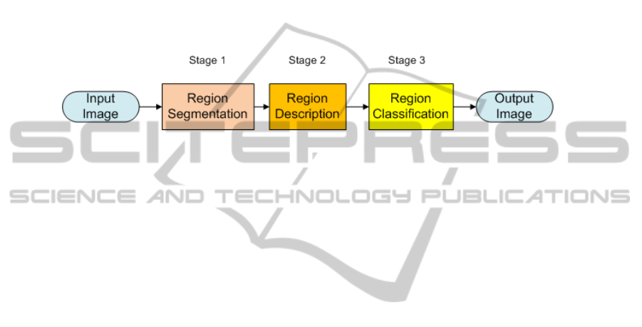
In order to achieve this goal we base our approach on a common Pattern Recognition

scheme (see Figure 1). The input to the scheme is a frame from a colonoscopy video

and the output will be this same image annotated in terms of polyp detection.

Fig. 1. General scheme of our approach.

The ﬁrst stage, Region Segmentation, consists of segmenting automatically the im-

age in order to end up with a reduced number of relevant regions, one of them containing

a polyp. So the objectives are twofold: reduce the number of regions that should be ana-

lyzed and indicate which are the non-informative regions on where not even the human

eye can distinguish anything and therefore there will be no need to analyze them later.

The second and third stages (Region Description and Classiﬁcation) are closely

related one to the other. Once we have a few regions from the segmentation stage, we

need to ﬁnd which features in these regions can denote the presence or not of a cancer

polyp. The objective of the second stage will be to ﬁnd a series of descriptors that

describe better what is a polyp region and what is not and, in the third stage, using the

knowledge acquired from the examples, classify the input regions into polyp-containing

candidates or not.

In order to develop and test our approach we rely on a database of thousands of

images extracted from 15 different videos of colonoscopy interventions.

The structure of this paper is as follows: In Section 2 we present our Region Seg-

mentation stage. In Section 3 we introduce the Region Description and Region Classi-

ﬁcation Stages. In Section 4 we present our preliminary experimental results. Finally,

in Section 5 we expose the main conclusions that have been extracted from this work

along with a presentation of the Future Work that we plan to do.

2 Region Segmentation

2.1 Our Model of Appearance of a Polyp

As we have mentioned before, we are dealing with colonoscopy images obtained from

real interventions videos. While observing the videos, we have found out that the light-

ing of the probe can give us hints about what is a polyp in an image. As the light

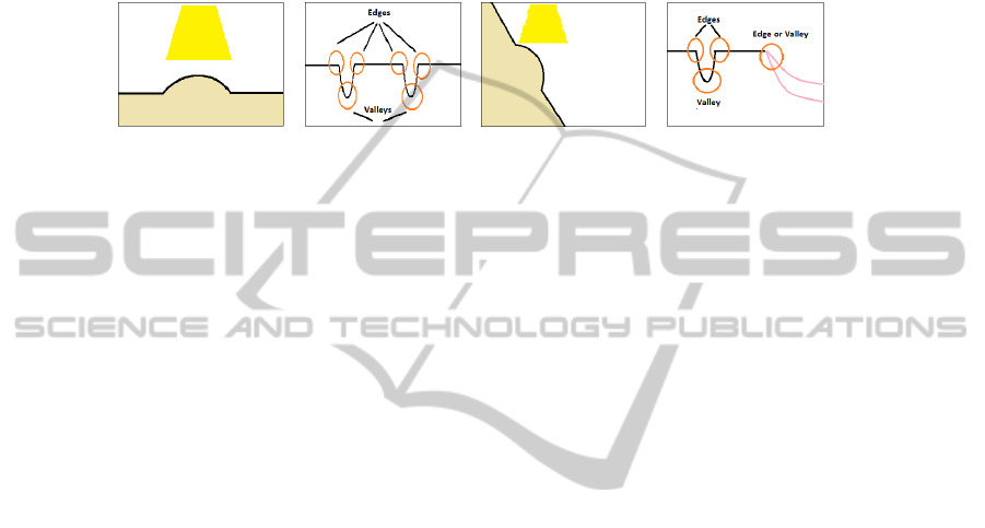
falls perpendicularly to the walls of the colon, it creates shadows around the surfaces

at which it is. More precisely, when the light falls into a prominent surface, it creates

a bright spot (with high grey-scale value) surrounded by darker areas, which are the

shadows, generating edges and valleys in the intensity image. This can be better under-

stood by looking at Figure 2, where we show an indication of the effect of light in the

intensity proﬁles, that depend on how the polyp appears (cenital or lateral view).

(a) (b) (c) (d)

Fig. 2. (a-b) Simulation of an overhead prominent surface and its correspondent grey-scale proﬁle

(c-d) Simulation of a lateral prominent surface and its correspondent grey-scale proﬁle.

Even considering this evidences of prominent surface appearance, there are some

challenges that need to be overcome:

– Non-uniform Polyp Appearance: ﬁrst, the appearance of the polyp by itself is not

uniform, going from peduncular to ﬂat shapes. Second, in most of the images we

will not have a clear vision of the polyp, viewing them from an overhead or lateral

views, which makes difﬁcult a shape-based recognition scheme work.

– Uniform Colour Pattern: as all the tissues in the image present a very similar color

distribution, a segmentation scheme based purely on color will have difﬁculties to

segment correctly the image.

– Effect of the Reﬂections, which makes segmentation algorithms create artiﬁcial

regions in the image.

– Over and under Segmentation: We can have two problems related to the number

of segmented regions. Oversegmentation is related to having a large number of

very small regions, which implies a high computation cost to analyze them all) and

under-segmentation to the fact of having a smaller number of bigger regions, but

still higher than the number of structures that a human could identify on the image).

Taking these considerations into account, we base our segmentation method on a

model of appearance of a polyp that we have deﬁned as a prominent shape enclosed

in a region that can be identiﬁed by the presence of edges and valleys. But we have to

take this as an indication, and we also should try to overcome the challenges we have

presented.

2.2 Region Segmentation Algorithm

In this subsection ﬁrst we present the basics of each step of our segmentation approach

and at the end we show in Figure 4, step by step, a complete graphical example.

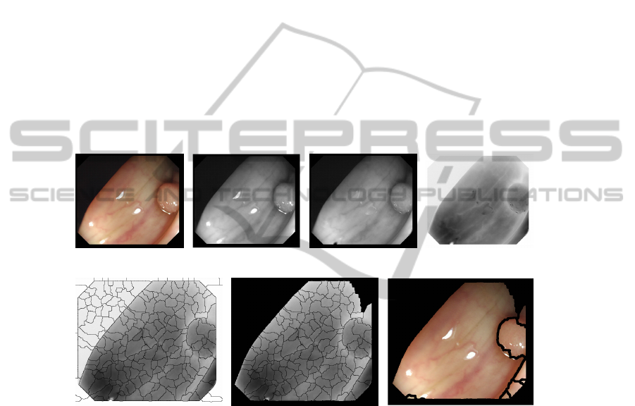
1. Image Preprocessing: Before applying any segmentation algorithm there are some

operations that should be done to the input image (Figure 4 a) in order to overcome

some of the challenges that were presented before. These preprocessing operations in-

clude: converting to gray-scale (Figure 4 b), image deinterleaving (as our images come

from a high deﬁnition interleaved video), correction of the reﬂections (Figure 4 c) and

obtaining the complemented version of the image (Figure 4 d).

2. Segmentation: In this step we have several alternatives. We can use either simpler

(in terms of computation cost) methods such as watersheds [5] or go with algorithms

that are more powerful in terms of segmentation such as Mean-shift or Normalized

Cuts. We use watersheds to reduce the computation cost and also because more complex

approaches are generally color-based which do not seem so useful in our case. Another

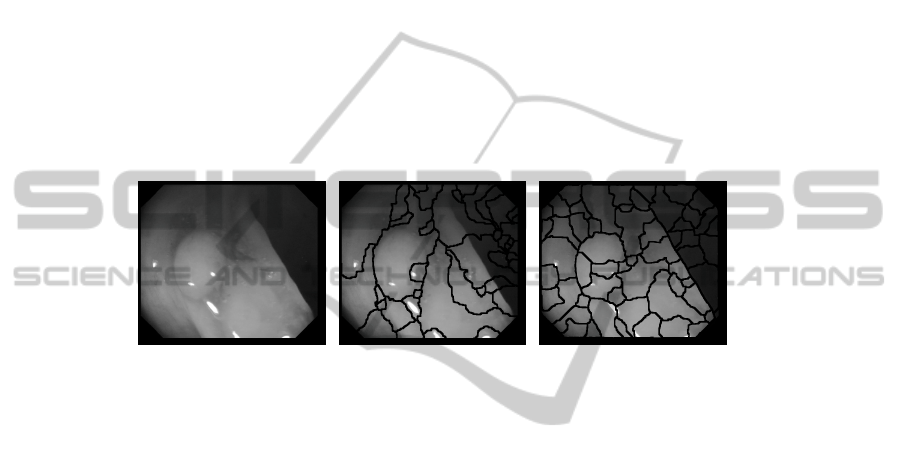
point of our approach is that, instead of using the preprocessed image obtained in the

ﬁrst step, we use gradient information, which, as it can be seen in Figure 3, encloses

better the structure of the shapes that appear on the image. After this step our image

will be divided in a large number of regions (Figure 4 e) that we will reduce by merging

them.

(a) (b) (c)

Fig. 3. (a) Original image (b) Original image segmentation (c) Gradient image segmentation.

3. Frontier-based Region Merging: in this step we focus on merging small neighbor

regions that are separated by weak frontiers (Figure 4 f). We denote as weak those

frontiers which present a low value of the weakness function (1).

F rontierW eakness = α ∗ edginess + β ∗ valleyness

+ γ ∗ anisotropic + η ∗ orientation

(1)

This weakness function is calculated using the response of the image to four different

weakness criteria: edges (by using a Canny detector the the image), valleyness (using a

ridges and valleys detector [6]), anisotropic ﬁltering and gradient-based orientation. For

each one of the criteria we create a binary mask and take as ﬁrst measure the percentage

of pixels that fall under the dark side of the mask. Once we have this percentage for each

of the criteria, we can decide if a frontier is weak according to a weakness criteria by

setting up a threshold.

We merge regions until there are no weak frontiers between regions (up to a thresh-

old value of the weakness function) or until the number of regions is stabilized.

4. Region-based Region Merging: in this step, as it did not happen in the previous

one, we consider when merging not only the weakness of the frontiers (by using a

different weakness function (2)) but also the grey-level content of the regions. In this

case the weakness measure takes into account which frontiers are kept after applying

consecutively two order-increasing median ﬁlters and a botton-hat mask.

F rontierW eakness = µ ∗ median + ρ ∗ bottom − hat (2)

Then we categorize the regions and frontiers, in terms of the amount of information

that they contain (i.e., low information means a region with a very high or very dark

mean grey level and very low standard deviation) and then merge compatible (same

kind of information) regions that have compatible weak frontiers. The objective here is

to end up with a reduced number of large regions as uniform as possible.

We merge regions until there are no weak frontiers between compatible regions (up

to a threshold weakness value) or until the number of regions is stabilized.

The objective of our segmentation and region merging sub-steps is twofold: ﬁrst ob-

taining a good segmentation of the image that ﬁts the structure of the several objects that

appear in it, such as polyps, and second, join and label those parts of the image where

we know we will not ﬁnd a polyp inside and therefore, we should not process them in

order to save resources. We show in Figure 4 one complete segmentation process.

(a) (b) (c) (d)

(e) (f) (g)

Fig. 4. (a) Original image (b) Grey-scale (c) Reﬂection corrected (d) Preprocessed image (e) First

segmentation (184 regions) (f) Before region-based merging (136 regions) (g) Final image (9

regions).

3 Region Description and Region Classiﬁcation

The objective of the Region Description stage is to choose a series of descriptors that

represent better what is a polyp region and what is not. We have made an study of the

bibliography of Feature Descriptors [7], dividing them into four groups: Shape Descrip-

tors, Color Descriptors, Texture Descriptors and Motion Descriptors. Our approach to

this stage is not to rely on one only type of descriptors and, as possible, try to use really

informative descriptors.

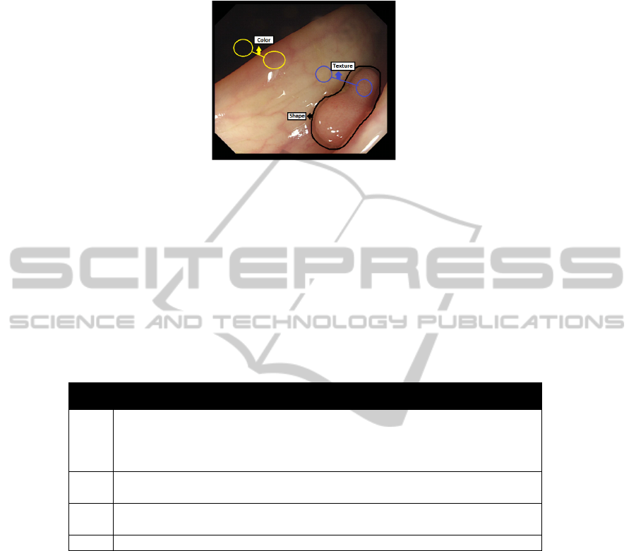
Fig. 5. Example of the need to use several types of descriptors.

If we take a look at the example, we can see that each of the types of descriptors

may have a role in our system. For example, we can see that the polyp is enclosed by a

closed contour and could be approximated by an ellipsoidal shape, so here we could use

Shape Descriptors. Color as it can be seen can be an important cue when deﬁning what

is clearly not a polyp and we can also observe the difference of Texture between the

polyp (more granular) and non-polyp regions (more plain). In Table 1 we show some of

the most important ones of each group.

Table 1. Examples of several feature descriptors.

Type Methods

Shape Contour-based: Global (Wavelets [8], Fourier [9], Shape Signature [10]) or Struc-

tural (Chain Code [11], Blurred Shape Model [12], Shape Context [13]).

Region-based: Global (Angular Radial Partitioning [14], Zernike Moments [15],

Shape Matrix [16]) or Structural (Skeletons).

Color Scalable Color Descriptor [17], Color Structure Descriptor [18], Color Constant

Color Indexing [19].

Texture SIFT [20], SURF [21], Texture Browsing Descriptor [22], Local Binary Patterns

[23], Co-ocurrence Matrices [24].

Motion Optical Flow [25], Angular Circular Motion [26].

Once we have described our regions we can start classifying them. As happens with

the Region Description step, this stage has not been implemented yet in our method be-

cause of two reasons: ﬁrst, time constraints (since we just started the development of our

approach) and secondly, and more important, because we have a strong belief in that the

classiﬁcation system is good as long as its inputs (outputs from the previous stages) are

good. As in many Pattern Recognition-based methods, we will use a machine learning

approach [27]. A learner can take advantage of examples (in our case, descriptions of

polyp and non-polyp containing regions) in order to capture characteristics of interest

of their unknown underlying probability distribution.

We will provide the system examples of regions that contain polyps and examples

of regions that no contain polyps. These example regions will be described and incor-

porated into the machine learning algorithm of choice in order to learn a polyp and

non-polyp pattern. New input images will be automatically segmented, described and

incorporated into the testing step with the objective of ﬁnding out if they are more near

to be a polyp candidate region or non-polyp candidate region. In our case our success

will be measured not only on terms of how many true positives we get but also on the

number of false negatives. It seems clear that it is harmless to identify one non-polyp

region as a polyp region that the opposite.

4 Experimental Results

4.1 Experimental Setup

In order to test the performance of our segmentation algorithm (because we have only

implemented the Region Segmentation stage until now) we have created a database

which consists of 150 different studies of polyp appearance in colonoscopy videos.

We have also a set of masks for each image (one that indicates the polyp position for

each image and another that indicates the non-informative regions) that will be used to

calculate the different performance measures.

We will use two different performance measures: Annotated Area Covered (AAC)

and Dice Similarity Coefﬁcient (DICE). The ﬁrst one indicates the maximum percent-

age of polyp that is contained on a single region while the second indicates, for the

region that covered more the polyp, the percentage of polyp information out of all the

region information. We will compare our method with Normalized Cuts [28] for both

polyp detection and non-informative region characterization.

4.2 Experimental Results

We show in Table 2 experimental results for both our method and Level Sets. The results

show that our approach is better than Normalized Cuts in terms of AAC but it is worse

than Normalized Cuts in terms of DICE, although our results for peduncular studies are

similar than the ones achieved by Normalized Cuts.

Table 2. Summary of the results.

Our Method Normalized Cuts

Measure /

Database

Whole Flat Peduncular Whole Flat Peduncular

Polyp AAC 96.5% 97.96% 92.79% 76.88% 79.33% 70.75%

Polyp DICE 22.07% 14% 42.23% 35.38% 28.10% 51.67%

Non-

informative

96.86% 96.46% 97.88% 80.38% 77.83% 86.71%

The reason for the great difference in DICE results lie on the fact that our method

divides the polyp area into smaller regions while Normalized Cuts ﬁts the polyp area in

a smaller number of regions. So in order to improve our results we should ﬁnd a way

to merge small polyp regions into bigger ones. We get better results than Normalized

Cuts in terms of AAC because our regions are smaller so they contain less both polyp

and non-polyp information and, in the case of a polyp region, as they are smaller, they

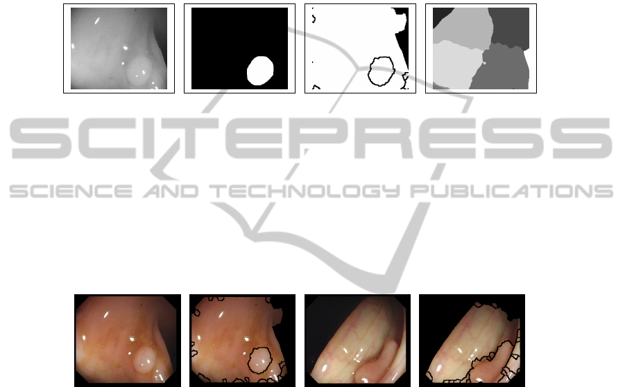
contain more polyp information. We show in Figure 6 qualitative segmentation results

(which have been calculated, for the sake of comparison, not taking into account the

black borders of the image). In general, the regions segmented by our method ﬁt better

the structure of the polyp but as they are smaller, they can miss some of the polyp

information. Normalized Cuts regions, as they are bigger, cover more polyp information

but they do not approximate well the shape of the polyp. Our method also gives better

results in terms of detecting which regions of the image are non-informative.

(a) (b) (c) (d)

Fig. 6. (a) Original images (b) Polyp mask (c) Final regions with our method (c) Final regions

with Normalized Cuts.

So, taking into account that Region Segmentation is only the ﬁrst stage of our ap-

proach (and that it is not ﬁnished yet) it seems clear that, if we are going to describe

later our regions to decide if they contain a polyp or not, our method is more suitable

than Normalized Cuts because our regions approximate better the polyp. To ﬁnish this

section we show in Figure 7 we show some preliminary qualitative segmentation re-

sults, that show that ﬁrst, we are reducing the search area of the image by eliminating

non-informative regions and second, that we end up with a low number of regions.

(a) (b) (c) (d)

Fig. 7. (a-c) Original images (b-d) Segmented images.

5 Conclusions

Our objective is to detect polyps in colonoscopy videos. To do so, we propose a Pattern

Recognition scheme divided in three main stages. The ﬁrst one, Region Segmentation,

is done with two objectives: reduce the size of the problem (as one of our possible

applications can be real-time polyp detection) as much as possible, and provide as result

to the later stages of the process chain a set of regions of interest. In order to segment

the image we have studied in depth the structure of several polyp-containing images

from our video database, with the aim of ﬁnding cues that can let us discern which

regions have some evidence of containing polyps and which not (in this case, we will

not analyze again these regions). So far, our method reduces greatly the number of

regions, offering as output a small number of them that, in some cases, cover the whole

shape of the polyp in just one region and, as the experimental results show, we identify

well the non-informative regions of the image.

Once we have this subset of regions of interest, the next step, Region Description,

will consist of describing them in terms of features to characterize them. This step will

be the seed to the ﬁnal stage, Region Classiﬁcation, where our plan is to implement

a machine learning approach. The ideal output will be a mask superimposed to the

image that indicates the region of the image that more likely contains a polyp. The

segmentation results give us hope that, after some improvements, we will be able to

start with the description step.

Acknowledgements

The authors would like to thank Dr. Antonio L

opez and Dr. Debora Gil for their helpful

comments and suggestions. This work was supported in part by a research grant from

Universitat Auton

oma de Barcelona 471-01-3/08, by the Spanish Government through

the founded project ”COLON-QA” (TIN2009-10435) and by research programme Con-

solider Ingenio 2010: MIPRCV (CSD2007-00018).

References

1. National Cancer Institute, “What You Need To Know About Cancer of the Colon and Rec-

tum,” U.S. National Institutes of Health, pp. 1–8, 2010.

2. A. Tresca, “The Stages of Colon and Rectal Cancer,” New York Times (About.com), p. 1,

2010.

3. J. Hassinger, S. Holubar, et al., “Effectiveness of a Multimedia-Based Educational Interven-

tion for Improving Colon Cancer Literacy in Screening Colonoscopy Patients,” Diseases of

the Colon & Rectum, vol. 53, no. 9, p. 1301, 2010.

4. National Digestive Diseases Information Clearinghouse, “Colonoscopy,” National Institute

of Diabetes and Digestive and Kidney Diseases (NIDDK), NIH, p. 1, 2010.

5. L. Vincent and P. Soille, “Watersheds in digital spaces: an efﬁcient algorithm based on

immersion simulations,” IEEE Transactions on Pattern Analysis and Machine Intelligence,

vol. 13, no. 6, pp. 583–598, 1991.

6. A. L

opez, F. Lumbreras, et al., “Evaluation of methods for ridge and valley detection,” IEEE

Transactions on Pattern Analysis and Machine Intelligence, vol. 21, no. 4, pp. 327–335,

1999.

7. J. Bernal, F. Vilari

no, and J. S

anchez, “Feature Detectors and Feature Descriptors: Where

Are Now,” Tech. Rep. 154, Computer Vision Center, Universitat Aut

onoma de Barcelona,

September 2010.

8. C. H. Chuang and C. C. J. Kuo, “Wavelet descriptor of planar curves: Theory and applica-

tions,” IEEE Transactions on Image Processing, vol. 5, no. 1, pp. 56–70, 2002.

9. H. Kauppinen, T. Seppanen, and M. Pietikainen, “An experimental comparison of autore-

gressive and Fourier-based descriptors in 2D shape classiﬁcation,” IEEE Transactions on

Pattern Analysis and Machine Intelligence, p. 201, 1995.

10. D. Zhang and G.Lu, “Review of Shape Representation and Description Techniques,” Pattern

Recognition, vol. 37, no. 1, pp. 1–19, 2004.

11. J. Sun and X. Wu, “Shape Retrieval Based on the Relativity of Chain Codes,” Lecture Notes

in Computer Science, Multimedia Content Analysis and Mining, vol. 4577/2007, pp. 76–84,

2007.

12. A. Forn

es and S. E. et al., “Handwritten Symbol Recognition by a Boosted Blurred Shape

Model with Error Correction,” Pattern Recognition and Image Analysis, pp. 13–21, 2007.

13. J. Bohg and D. Kragic, “Grasping Familiar Objects Using Shape Context,” in International

Conference on Advanced Robotics. ICAR 2009, pp. 1–6, June 2009.

14. A. Chalechale, A. Mertins, and G. Naghdy, “Edge image description using angular radial

partitioning,” IEEE Proceedings-Vision Image and Signal Processing, vol. 151, no. 2, pp. 93–

101, 2004.

15. A. Khotanzad and Y. H. Hong, “Invariant Image Recognition by Zernike Moments,” IEEE

Transactions on Pattern Analysis and Machine Intelligence, vol. 12, pp. 489–497, 1990.

16. D. Zhang and M. C. Y. Lim, “An efﬁcient and robust technique for region based shape

representation and retrieval,” in 6th IEEE/ACIS International Conference on Computer and

Information Science, 2007. ICIS 2007, pp. 801–806, 2007.

17. D. Borghesani, C. Grana, and R. Cucchiara, “Color Features Performance Comparison for

Image Retrieval,” Image Analysis and Processing–ICIAP 2009, pp. 902–910, 2009.

18. M. Kundu, M. Banerjee, and P. Bagrecha, “Interactive Image Retrieval in a Fuzzy Frame-

work,” Fuzzy Logic and Applications, vol. 5571, pp. 246–253, 2009.

19. B. V. Funt and G. D. Finlayson, “Color Constant Color Indexing,” IEEE Transactions on

Pattern Analysis and Machine Intelligence, vol. 17, no. 5, pp. 522–529, 1995.

20. D. G. Lowe, “Object Recognition from Local Scale-Invariant Features,” in International Con-

ference on Computer Vision, Corfu, Greece, pp. 1150–1157, Published by the IEEE Com-

puter Society, 1999.

21. H. Bay, T. Tuytelaars, and L. V. Gool, “SURF: Speeded Up Robust Features,” Computer

Vision–ECCV 2006, pp. 404–417, 2006.

22. K. L. Lee and L. H. Chen, “An efﬁcient computation method for the texture browsing de-

scriptor of MPEG-7,” Image and Vision Computing, vol. 23, no. 5, pp. 479–489, 2005.

23. T. Ojala, M. Pietikainen, and T. Maenpa, “Gray scale and rotation invariant texture classiﬁ-

cation with local binary patterns,” Computer Vision-ECCV 2000, pp. 404–420, 2000.

24. J. R. Carr and F. P. de Miranda, “The semivariogram in comparison to the co-occurrence

matrix for classiﬁcation of image texture,” IEEE Transactions on Geoscience and Remote

Sensing, vol. 36, pp. 1945–1952, nov 1998.

25. B. K. P. Horn and B. G. Schunck, “Determining Optical Flow,” Artiﬁcial Intelligence,

vol. 17, no. 1-3, pp. 185–203, 1981.

26. B. Erol and F. Kossentini, “Local Motion Descriptors,” in IEEE Workshop on Multimedia

Signal Processing, vol. October 2001, pp. 467–472, 2001.

27. C. Bishop et al., Pattern recognition and machine learning. Springer New York, 2006.

28. J. Shi and J. Malik, “Normalized cuts and image segmentation,” Pattern Analysis and Ma-

chine Intelligence, IEEE Transactions on, vol. 22, no. 8, pp. 888–905, 2002.