MEAN SHIFT OBJECT TRACKING USING A 4D KERNEL AND
L
INEAR PREDICTION
Katharina Quast, Christof Kobylko and Andr´e Kaup
Multimedia Communications and Signal Processing, University of Erlangen-Nuremberg
Cauerstr. 7, 91058 Erlangen, Germany
Keywords:
Object tracking, Mean shift tracking.
Abstract:
A new mean shift tracker which tracks not only the position but also the size and orientation of an object is
presented. By using a four-dimensional kernel, the mean shift iterations are performed in a four-dimensional
search space consisting of the image coordinates, a scale and an orientation dimension. Thus, the enhanced
mean shift tracker tracks the position, size and orientation of an object simultaneously. To increase the tracking
performance by using the information about the position, size and orientation of the object in the previous
frames, a linear prediction is also integrated into the 4D kernel tracker. The tracking performance is further
improved by considering the gradient norm as an additional object feature.
1 INTRODUCTION
Object tracking is still an important and challenging
task in computer vision. Among the many different
methods developed for object tracking, the mean shift
algorithm (Comaniciu and Meer, 2002) is one of the
most famous tracking techniques, because of its ease
of implementation, computational speed, and robust
tracking performance. Besides, mean shift tracking
doesn’t require any training data as learning based
trackers like (Kalal et al., 2010). In spite of its ad-
vantages, traditional mean shift suffers from the lim-
itations of the use of a kernel with a fixed band-
width. Since the scale and the orientation of an object
changes over time, the bandwidth and the orientation
of the kernel profile should be adapted accordingly.
An intuitive approach for adapting the kernel
scale is to run the algorithm with three different ker-
nel bandwidths, former bandwidth and former band-
width ± 10%, and to choose the kernel bandwidth
which maximizes the appearance similarity (±10%
method) (Comaniciu et al., 2003). A more sophisti-
cated method using difference of Gaussian mean shift
kernel in scale space has been proposed in (Collins,
2003). The method provides good tracking results,
but is computationally very expensive.
Mean shift based methods which are adapting the
scale and the orientation of the kernel are presented
in (Bradski, 1998; Qifeng et al., 2007). In (Bradski,
1998) scale and orientation of a kernel are obtained
by estimating the second order moments of the object
silhouette, but that is of high computational costs. In
(Qifeng et al., 2007) adaptation of the kernel scale and
orientation is achieved by combining the mean shift
method with adaptive filtering, which is based on the
recursive least squares algorithm.
In this paper we propose a scale and orientation
adaptivemean shift tracker, which doesn’t require any
other iterative or recursive method nor destroys the
realtime capability of the tracking process. This is
achieved by tracking the target in a virtual 4D search
space considering the position coordinates as well as
the target scale and rotation angle as additional di-
mensions. The tracking method is further enhanced
by a linear prediction of the object scene parameters
(position, scale and orientation) and by using the im-
age gradient norm as an additional object feature.
The rest of the paper is organized as follows. Sec-
tion 2 gives an overview of standard mean shift track-
ing. Mean shift tracking in the 4D search space is
explained in Section 3. While the linear prediction is
described in Section 4 and the image gradient norm
is introduced in Section 5. Experimental results are
shown in Section 6. Section 7 concludes the paper.
2 MEAN SHIFT OVERVIEW
Mean shift tracking discriminates between a target
model in frame n and a candidate model in frame
n + 1. The target model is estimated from the dis-
588
Quast K., Kobylko C. and Kaup A..
MEAN SHIFT OBJECT TRACKING USING A 4D KERNEL AND LINEAR PREDICTION.
DOI: 10.5220/0003327305880593
In Proceedings of the International Conference on Computer Vision Theory and Applications (VISAPP-2011), pages 588-593
ISBN: 978-989-8425-47-8
Copyright
c
 2011 SCITEPRESS (Science and Technology Publications, Lda.)

crete density of the objects feature histogram q(ˆx) =
{q
u
(ˆx)}
u=1...m
with
∑
m
u=1
q
u
(ˆx) = 1.
The probability of a certain feature belonging to
the object with the centroid ˆx is expressed as q
u
(ˆx),
which is the probability of the feature u = 1...m oc-
curring in the target model. The candidate model
p(ˆx
new
)is defined analogous to the target model, for
more details see (Comaniciu and Meer, 2002; Co-
maniciu et al., 2003). The mean shift algorithm com-
putes the offset from an old object position ˆx to a new
position ˆx
new
= ˆx + ∆x by estimating the mean shift
vector
∆x =
∑
i
K(x
i
− ˆx)w(x
i
)(x
i
− ˆx)
∑
i
K(x
i
− ˆx)w(x
i
)
(1)
with kernel K(·) and weighting function w(x
i
) which
denotes the weight of x
i
as
w(x
i
) =
m
∑
u=1
δ[b(x
i
) − u]
s
q
u
(ˆx)
p
u
(ˆx
new
)
. (2)
The similarity between target and candidate model
is measured by the discrete formulation of the Bhat-
tacharyya coefficient
ρ[p(ˆx
new
),q(ˆx)] =
m
∑
u=1
p
p
u
(ˆx
new
)q
u
(ˆx). (3)
The aim is to minimize the distance between the two
color distributions d(ˆx
new
) =
p
1− ρ[p(ˆx
new
),q(ˆx)]
as a function of ˆx
new
in the neighborhood of a given
position ˆx
0
. This can be achievedusing the mean shift
algorithm. By running this algorithm the kernel is re-
cursively moved from ˆx
0
to ˆx
1
according to the mean
shift vector.
3 4D KERNEL TRACKING
3.1 4D Kernel Definition
Usually a scaled Epanechnikov kernel is used for
mean shift tracking which is defined as
K
e
(x) =
1
h
d
· k
e

kxk
2
h
2

(4)
where h is the kernel bandwith and k
e
the profile of the
radially symmetric Epanechnikov kernel as defined in
equation (12) in (Comaniciu et al., 2003).
Since a radially symmetric kernel is usually a bad
approximation of the tracked object shape, we are
using an elliptic kernel with varying bandwidths for
both semi-axes, which is scaled by a scaling factor s
and rotated by a rotation angle φ:
K
′
(x,s, φ) =
1
h
a
· h
b
· s
2
· k
′

kH· R(ϕ + φ)·xk
2
s
2

(5)
Normalized x - Coordinate
Scale
-1
-0.5 0 0.5 1
-1.4
-1.3
-1.2
-1.1
-1
-0.9
-0.8
-0.7
-0.6
Figure 1: Cut surface of the adaptive kernel with the x-
scale-plane when only scale adaptation is used. The col-
ors correspond to the kernel-weights where dark-blue rep-
resents 0 and dark-red represents the maximum kernel-
weight.
where k
′
is the kernel profile, h
a
and h
b
are the band-
widths for the semi-major and semi-minor axis, and ϕ
being the rotation angle between the semi-major axis
and the horizontal coordinate axis of the image. The
scaling matrix H and the rotation matrix R are defined
as follows:
H =
1
h
a
0
0
1
h
b
!
(6)
R(ϕ) =

cos(ϕ) −sin(ϕ)
sin(ϕ) cos(ϕ)

(7)
The scaled and rotated kernels K
′
(·) are considered to
be the cut surfaces of a 4D tracking kernel with the
2D image plane. As position, scale and rotation are
considered to be linearly independent, the scale and
orientation adaptive 4D kernel is defined by:
K
a
(x,s, φ) = K
′
(x,s,φ) · K
e

s− 1
h
s

· K
e

φ
h
φ

(8)
with 1D Epanechnikov kernels with the bandwidth h
s
for the scale dimension and the bandwidth h
φ
for the
rotation dimension. Since the target scale is updated
multiplicatively and the target rotation additively, the
scale kernel is centered at one (neutral element for
multiplication) and the rotation kernel at zero (neutral
element for addition). Figure 1 shows the cut surface
of the adaptive kernel with the plane spaned by the
normalized x-coordinate and the scale dimension if
only scale adaptation is used.
3.2 Tracking in the 4D Space
In order to run the mean shift tracking with the 4D
kernel K
a
(·), the kernel has to be sampled in the scale
and rotation dimension and thus a set of N
s
·N
φ
scaled
and rotated kernels K
′
(·) is being constructed. An ex-
ample of the resulting kernel-weights for an uniform
MEAN SHIFT OBJECT TRACKING USING A 4D KERNEL AND LINEAR PREDICTION
589

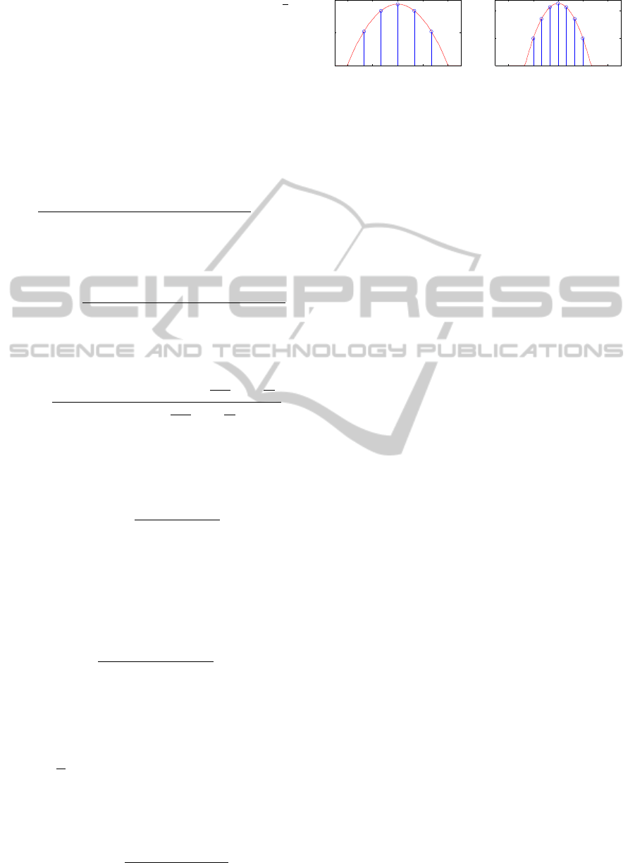
sampling with N
s
= 5, h
s
= 0.4, N
φ
= 7 and h
φ
=
π
6
is shown in Figure 2. Of course, each of this kernels
covers a different area and, therefore, each one has its
own pixel set {x
i
}
i=1..n
h
(s
k
,φ
m
)
for the kernel density
estimation (KDE).
Using the whole kernel set centered at y, the can-
didate histogram is estimated by:
ˆp[u](y) =C
a
·
N
s
∑
k=1
N
φ
∑
m=1
n
h
(s
k
,φ
m
)
∑
i=1
K
a
(y−x
i
,s
k
,φ
m
)·δ[b(x
i
) − u]
(9)
with the normalization constant
C
a
=
1
∑
N
s
k=1
∑
N
φ
m=1
∑
n
h
(s
k
,φ
m
)
i=1
K
a
(y− x
i
,s
k
,φ
m
)
(10)
Basically, the 4D KDE equals a series of 2D KDEs
with the scaled and rotated kernels:
ˆp[u](y,s
k
,φ
m
) =
∑
n
h
(s
k
,φ
m
)
i=1
K
′
(y− x
i
,s
k
,φ
m
) · δ[b(x
i
) − u]
∑
n
h
(s
k
,φ
m
)
i=1
K
′
(y− x
i
,s
k
,φ
m
)
(11)
with a posterior averaging of all separately computed
histograms:
ˆp[u](y) =
∑
N
s
k=1
∑
N
φ
m=1
ˆp[u](y,s
k
,φ
m
) · K
e
(
s
k
−1
h
s
) · K
e
(
φ
m
h
φ
)
∑
N
s
k=1
∑
N
φ
m=1
K
e
(
s
k
−1
h
s
) · K
e
(
φ
m
h
φ
)
(12)
Since a high pixel-weight w(x
i
) means a high
probability of the pixel x
i
belonging to the target, the
mean pixel-weight
¯w(s
k
,φ
m
) :=
∑
n
h
(s
k
,φ
m
)
i=1
w(x
i
)
n
h
(s
k
,φ
m
)
(13)
inside the area covered by the kernel K
′
(x,s
k
,φ
m
) de-
picts how well the target is approximated by this par-
ticular kernel.
The overall mean pixel-weight of the kernel set is
then defined by:
¯w :=
∑
N
s
k=1
∑
N
φ
m=1
¯w(s
k
,φ
m
)
N
s
· N
φ
(14)
Thus, the new candidate position is averaged over
all kernels of the set, favoring these which approxi-
mate the target better.
ˆy
1
=
1
¯w
·
N
s
∑
k=1
N
φ
∑
m=1
¯w(s
k
,φ
m
) · ˆ
y
1
(s
k
,φ
m
) (15)
with ˆy
1
(s
k
,φ
m
) being the new candidate position com-
puted with one particular kernel of the set:
ˆy
1
(s
k
,φ
m
) =
∑
n
h
(s
k
,φ
m
)
i=1
x
i
· w(x
i
)
∑
n
h
(s
k
,φ
m
)
i=1
w(x
i
)
(16)
kernel weight
kernel weight
kernel scale s
kernel rotation φ
4/π
2/π
-π/4
-π/8
0
0
0
1
1
2
0.6
0.8
1.2
1.4
π/4
π/8
Figure 2: Sampling of scale (left) and rotation (right) di-
mension. The continuous kernel is depicted by the red
curve.
Once the final target position has been found, the
scale and rotation angle update-values are computed
by one mean shift iteration in the proper dimensions:
ˆs = (1/ ¯w) ·
∑
N
s
k=1
s
k
·
∑
N
φ
m=1
¯w(s
k
,φ
m
)
ˆ
φ = (1/ ¯w) ·
∑
N
φ
m=1
φ
m
·
∑
N
s
k=1
¯w(s
k
,φ
m
)
(17)
Usually, this should be done after each candidate
position update, but it would require a reconstruction
of the entire kernel set after each iteration. Since the
linear approximation of the scale and rotation angle
update-value has proven to be quite sufficient in the
experiments, this compromise has been made in re-
spect to computational efficiency.
Finally, the target scale and rotation angle are up-
dated by:
h
′
a
= h
a
· ˆs
h
′
b
= h
b
· ˆs
ϕ
′
= ϕ+
ˆ
φ
(18)
4 LINEAR PREDICTION OF THE
OBJECT SCENE PARAMETERS
Like all iterative solution techniques, the mean shift
procedure requires the initial guess (target position in
the last image) to be sufficiently close to the sought
extremum (current target position) for convergence.
Under perfect circumstances this means that the track-
ing kernels have to overlap, but if the tracked object
is moving too fast or the scene is captured with a low
frame rate that might not be the case. Fortunately, the
changes of the object scene parameters are partly pre-
dictable. Due to the fact that the overall scene param-
eters (e.g. real-world position of object and camera)
are not known in general, we concentrated on a ba-
sic linear prediction rather than on a prediction based
on a physical movement model like the one using a
Kalman-filter mentioned in (Comaniciu et al., 2003).
The simplest kind of linear prediction would be to
assume that the current change of the object scene pa-
rameters equals to the last one. Usually, this would be
a good guess since the velocity of the object does not
change drastically during the sampling interval of the
VISAPP 2011 - International Conference on Computer Vision Theory and Applications
590

camera, but this estimation would be highly suscepti-
ble to noisy input data, because only one data point is
being used for the estimation. The influence of the in-
put noise, however, can be minimized by computing
the mean-value of the most recent data points, assum-
ing that the object scene parameters do not change
much during the considered interval.
For the computation of the mean-value, one has
to distinguish between additively or multiplicatively
updated parameters P. In general, if N
P
previous pa-
rameter updates ∆P
i
are being regarded for the mean-
value computation, then a consecutive update by all
∆P
i
must equal a N
P
-fold update by the mean-value
c
∆P. Let P
t
be the parameter at time index t and ∆P
t
the parameter update between the time indices t and
t + 1:
Additive updates are defined by
ˆ
P
t
= P
t−N
P
+
N
P
∑
i=1
∆P
t−i
= P
t−N
P
+ N
P
·
c
∆P
t
. (
19)
Thus, the predicted update-value equals the arithmetic
mean:
c
∆P
t
=
1
N
P
·
N
P
∑
i=1
∆P
t−i
(20)
Multiplicative updates, on the other hand, are de-
fined by
ˆ
P
t
= P
t−N
P
·
N
P
∏
i=1
∆P
t−i
= P
t−N
P
·
c
∆P
N
P
t
(
21)
resulting in the geometric mean being the predicted
update-value:
c
∆P
t
=
N
P
v
u
u
t
N
P
∏
i=1
∆P
t−i
(22)
Applying the logarithm on both sides of equation
(22) transforms the geometric mean of the update-
value into an arithmetic mean of its logarithmic value:
ln
c
∆P =
1
N
P
·
N
P
∑
i=1
ln∆P
t−i
(23)
Therefore, the same prediction method can be used
for both types of parameter updates.
Since the position y as well as the rotation angle
ϕ are updated additively, while the kernel bandwidth
(h
a
,h
b
)
T
is updated multiplicatively by the scale fac-
tor s, the vector of the changes of the object scene
parameters at the time index t is defined by
p
t
=



∆y
1
[t]
∆y
2
[t]
lns[t]
φ[t]



(24)
and the parameter changes in the current image are
estimated by computing the arithmetic mean of the
preceding parameter changes:
ˆ
p
t
=
1
N
P
·
N
P
∑
i=1
p
t−i
(25)
Before performing the mean shift iterations, the
object scene parameters found in the last image are
updated using the estimated changes:
ˆy
0
[t] = y
0
[t] +
d
∆y
1
[t]
d
∆y
2
[t]
!
(26)

ˆ
h
a
[t]
ˆ
h
b
[t]

=

h
a
[t]
h
b
[t]

· e
ln ˆs[t]
(27)
ˆ
ϕ[t] = ϕ[t] +
ˆ
φ[t] (28)
5 ADDITIONAL FEATURES
Obviously, the color distribution is a very attractive
feature, because it is usually very distinctive and it is
offered to the tracker without the need of further im-
age processing. Since the KDE works pixel-based,
the tracker would benefit from any feature providing
information about the correlation between neighbor-
ing pixels. However, using the oriented image gra-
dients, computed by the Sobel filter, directly as ad-
ditional features would be problematic. This would
triple the number of image features, aggravating the
curse of dimensionality (Scott, 1992) and disturbing
the comparison between the target and the candidate
histogram. Furthermore, the histogram would be-
come highly rotation-variant and the tracker could be
very easily mislead by changes of the object pose.
A possible solution would be to use only the norm
of the combined image gradient vector as a new fea-
ture. Unlike one might think, this does not result in a
huge loss of information as the individual color plane
gradients are highly correlated anyway, because they
appear mainly at object contours. In respect to com-
putational efficiency, the L1 norm is being used.
I
M+1
(x) = k [ (∇I
1
(x))
T
,.., (∇I
M
(x))
T
]
T
k
1
(29)
with I
l
being the l-th feature plane of the image and
kxk
1
:=
dim(x)
∑
i=1
|x
i
|. (
30)
6 EXPERIMENTAL RESULTS
For estimating the target histogram each color chan-
nel of the RGB space as well as the image gradi-
ent norm is quantized into 8 bins, leading to a to-
tal of 8
4
= 4096 different histogram bins. The used
MEAN SHIFT OBJECT TRACKING USING A 4D KERNEL AND LINEAR PREDICTION
591

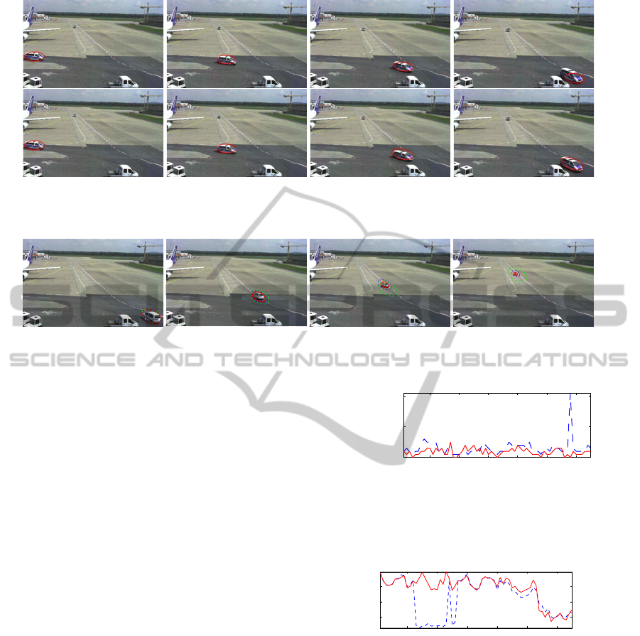
Figure 3: Results for tracking a police car in sequence Airport using the proposed method without gradient information (top)
and with gradient information (bottom).
Figure 4: Results for tracking a white car in sequence Airport using the standard mean shift (green) and the proposed method
with scale and rotation adaptation (blue) and with parameter prediction and scale and rotation adaptation (red).
adaptation parameters were set to h
s
= 0.4, h
φ
= 30
◦
,
N
s
= 5 and N
φ
= 5. Thus, the enhanced mean shift
tracker was run in the 4D space with a kernel set of
N
s
· N
φ
= 25 kernels.
In the sequence Airport (3 fps) vehicles which are
moving on an airport apron were tracked using the
standard mean shift tracker as well as the proposed
enhanced mean shift tracker. In Figure 3 the results of
the proposed tracker tracking a police car in sequence
Airport with and without using the gradient informa-
tion is shown. It can be seen, that the gradient infor-
mation is an useful object feature, because the size of
the police car is tracked much more reliably using the
gradient information. Thus, for all other experiments
the gradient information is used for all trackers.
In Figure 4 the results of the standard mean shift
method are compared to the proposed method with
and without using the linear prediction of the ob-
ject scene parameters. While the standard mean shift
tracker is not able to adapt to the orientation and size
of the car (top row) in Figure 4, the new 4D kernel
tracker is able to track the size as well as the orienta-
tion (middle row) of Figure 4. The results can even be
further enhanced by using the linear prediction (bot-
tom row) of Figure 4.
To demonstrate the strength of the adaptive mean
shift tracker for tracking fast moving objects, the
tracking performance is also evaluated using the se-
quence Table Tennis (30 fps). Since the orientation
adaptation is not needed for tracking a circular object
like a ball, N
φ
was set to 1. The results for the standard
Frame
Iterations
10
20 30 40 50 60
0
10
20
Figure 5: Mean shift iterations needed by the standard mean
shift tracking (dashed blue) and by the proposed enhanced
mean shift tracking (solid red) for the sequence Table Ten-
nis.
Frame
ρ
10 20 30 40
50
60
0.6
0.7
0.8
Figure 6: Bhattacharyya Coefficient ρ of the standard mean
shift tracking (dashed blue) and of the proposed enhanced
mean shift tracking (solid red) for the sequence Table Ten-
nis.
mean shift tracker and the proposed tracker can be
seen in Figure 7. The number of mean shift iterations
needed is shown in Figure 5. Both methods do not re-
quire many iterations, but in most cases the proposed
enhanced mean shift algorithm needs less iterations
than the standard method. Especially around frame
60, when the ball is partly occluded, the proposed
tracker needs less iterations than the standard tracker.
The Bhattacharyya coefficient of the enhanced mean
shift tracker is also more reliable than the one of
VISAPP 2011 - International Conference on Computer Vision Theory and Applications
592

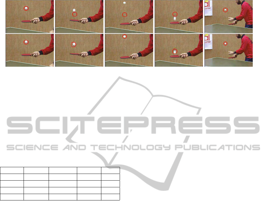
Figure 7: Tracking results for sequence Table Tennis of standard mean shift (top) and of the proposed method with scale and
rotation adaptation (bottom).
the standard method, see Figure 6. Especially be-
tween the frames 13 to 27 the Bhattacharyya coeffi-
cient of the standard mean shift tracker decreases and
becomes unreliable, because the standard mean shift
tracker is not able to follow the fast movement of the
ball. While, the proposed tracker has a high and there-
with reliable Bhattacharyya coefficient.
Table 1: Computational performance for tracking the po-
lice car in sequence Airport and the ball in sequence Table
Tennis.
Tracker Target Kernel size Iterations fps
standard police car 97x45 6.63 76.77
proposed police car 100.7x46.8 3.87 4.22
standard ball 33x33 3.02 430.48
proposed ball 31.4x31.4 1.82 97.81
In Table 1 the computational performance, the av-
erage kernel size in pixels and the average number
of mean shift iterations of both trackers are given.
Although the enhanced tracker runs with 25 kernels
for sequence Airport, 5 for sequence Table Tennis re-
spectively, it performs in in real-time. However, it is
slower as the standard mean shift tracker.
7 CONCLUSIONS
A new mean shift tracking method using an adaptive
4D kernel to perform the mean shift iterations in an
extended 4D search space has been proposed. Thus,
the tracker adapts to the changing object scene param-
eters. Compared to the standard mean shift algorithm,
which only tracks the position, the proposed tracker is
able to track the position as well as the scale and the
orientation of an object. The flexibility of the adap-
tation can be adjusted by the sampling scheme of the
scale and rotation dimensions to match the individual
requirements of each tracking scenario. By using the
L1 norm as an additional feature the performance is
further enhanced. Future work might concentrate on
getting the tracker even more robust especially against
background clutter.
ACKNOWLEDGEMENTS
This work has been supported by the Gesellschaft f¨ur
Informatik, Automatisierung und Datenverarbeitung
(iAd) and BMWi, ID 20V0801I.
REFERENCES
Bradski, G. (1998). Computer vision face tracking for use in
a perceptual user interface. Intel Technology Journal,
2:12–21.
Collins, R. T. (2003). Mean-shift blob tracking through
scale space. In Proc. IEEE Computer Society Con-
ference on Computer Vision and Pattern Recognition,
volume 2, pages 234–240.
Comaniciu, D. and Meer, P. (2002). Mean shift: A robust
approach toward feature space analysis. IEEE Trans-
actions on Pattern Analysis and Machine Intelligence,
24:603–619.
Comaniciu, D., Ramesh, V., and Meer, P. (2003). Kernel-
based object tracking. IEEE Transactions on Pattern
Analysis and Machine Intelligence, 25:564–575.
Kalal, Z., Matas, J., and Mikolajczyk, K. (2010). PN learn-
ing: Bootstrapping binary classifiers by structural
constraints. In Computer Vision and Pattern Recogni-
tion (CVPR), 2010 IEEE Conference on, pages 49–56.
IEEE.
Qifeng, Q., Zhang, D., and Peng, Y. (2007). An adaptive
selection of the scale and orientation in kernel based
tracking. In Proc. IEEE Conference on Signal-Image
Technologies and Internet-Based Systems, pages 659–
664.
Scott, D. W. (1992). Multivariate Density Estimation: The-
ory, Practice, and Visualization. Wiley-Interscience.
MEAN SHIFT OBJECT TRACKING USING A 4D KERNEL AND LINEAR PREDICTION
593