PROXIMITY-BASED GRAPH EMBEDDINGS FOR MULTI-LABEL

CLASSIFICATION

Tingting Mu and Sophia Ananiadou

National Centre for Text Mining, University of Manchester, 131 Princess Street, Manchester, M1 7DN, U.K.

Keywords:

Dimensionality reduction, Embedding, Supervised, Adjacency graph, Multi-label classiﬁcation.

Abstract:

In many real applications of text mining, information retrieval and natural language processing, large-scale

features are frequently used, which often make the employed machine learning algorithms intractable, leading

to the well-known problem “curse of dimensionality”. Aiming at not only removing the redundant informa-

tion from the original features but also improving their discriminating ability, we present a novel approach

on supervised generation of low-dimensional, proximity-based, graph embeddings to facilitate multi-label

classiﬁcation. The optimal embeddings are computed from a supervised adjacency graph, called multi-label

graph, which simultaneously preserves proximity structures between samples constructed based on feature and

multi-label class information. We propose different ways to obtain this multi-label graph, by either working in

a binary label space or a projected real label space. To reduce the training cost in the dimensionality reduction

procedure caused by large-scale features, a smaller set of relation features between each sample and a set of

representative prototypes are employed. The effectiveness of our proposed method is demonstrated with two

document collections for text categorization based on the “bag of words” model.

1 INTRODUCTION

In information retrieval (IR), text mining (TM) and

natural language processing (NLP), research on how

to automatically generate a small set of informative

features from large-scale features, such as bag of n-

grams, are of increasing interest. The goal is not only

to reduce the computational cost but also to improve

the performance of a followed learning task, which

corresponds to the signiﬁcant problem of dimension-

ality reduction (DR) in machine learning. Relevant

reduction techniques commonly used by IR, TM and

NLP researchers include feature selection using wrap-

per or ﬁlter models (Lewis, 1992; Bekkerman et al.,

2003; Li et al., 2009), feature clustering (Bekkerman

et al., 2003; Dhillon et al., 2003), and latent variable

models (Deerwester et al., 1990; Blei et al., 2003).

More sophisticated research for DR has been

developed via manifold learning, multidimensional

scaling and spectral analysis. These methods gener-

ate low-dimensional embeddings so that they preserve

certain properties of the original high-dimensional

data. Different properties are usually quantiﬁed by

different objective functions, and the DR problem

can thus be formulated as an optimization problem

(Kokiopoulou and Saad, 2007). For instance, princi-

pal component analysis (PCA) (Jolliffe, 1986) pre-

serves the global structure of the data by maximiz-

ing the variance of the projected embeddings. Lo-

cally linear embedding (LLE) (Roweis and Saul,

2000) and orthogonal neighborhood preserving pro-

jections (ONPP) (Kokiopoulou and Saad, 2007) pre-

serve the intrinsic geometry at each neighborhood by

minimizing a reconstruction error. Spectral cluster-

ing (SC) analysis (Chan et al., 1994; Shi and Ma-

lik, 2000; Luxburg, 2007), Laplacian eigenmaps (LE)

(Belkin and Niyogi, 2003), locality preserving pro-

jection (LPP) (He and Niyogi, 2003), and orthogonal

LPP (OLPP) (Kokiopoulou and Saad, 2007) preserve

a certain afﬁnity graph constructed from the original

data by minimizing the penalized distances between

the embeddings of adjacent points. These methods

work in an unsupervised manner, which only preserve

the data property in the feature space. Although the

unsupervised reduction provides a compact represen-

tation of the data, when it is used as a preprocessing

step followed by a classiﬁcation task, it may not al-

ways improve the ﬁnal performance.

When there is extra label (class, category)

information available, it is natural to pursue

supervised/semi-supervised DR to improve the classi-

ﬁcation performance. Various DR research has been

Mu T. and Ananiadou S..

PROXIMITY-BASED GRAPH EMBEDDINGS FOR MULTI-LABEL CLASSIFICATION.

DOI: 10.5220/0003092200740084

In Proceedings of the International Conference on Knowledge Discovery and Information Retrieval (KDIR-2010), pages 74-84

ISBN: 978-989-8425-28-7

 2010 SCITEPRESS (Science and Technology Publications, Lda.)

conducted for single-label classiﬁcation task, where

each given sample belongs to only one class (He,

2004; Cai et al., 2007a; Yan et al., 2007; Zhang et al.,

2007; Kokiopouloua and Saadb, 2009; Sugiyama,

2007; Sugiyama, 2010). Among these methods,

Fisher discriminant analysis (FDA) (Fisher, 1936) is

the most popular one, which maximizes the between-

class scatter while minimizes the within-class scatter

of the projected embeddings. These methods work in

a similar way of minimizing the penalized distances

between the adjacent embeddings, of which the only

difference lies on the construction of an adjacency

graph and a constraint matrix. Single-label graphs are

employed in above methods, where the adjacency is

non-zero only when the two points belong to the same

class.

Recently, multi-label classiﬁcation becomes a re-

quirement in NLP, TM and bioinformatics, such as

text categorization (Zhang et al., 2008; Tang et al.,

2009) and protein function prediction (Barutcuoglu

et al., 2006). It allows the given samples to belong

to multiple classes. In this case, the above single-

label DR methods become inapplicable as there is

no clear deﬁnition of two samples belonging to the

same class, e.g. some of the classes two samples be-

long to are the same, but not all. Thus, to perform

supervised/semi-supervised DR for multi-label classi-

ﬁcation, one needs to avoid to incorporate such a deﬁ-

nition into the computation. Instead, some existing re-

search focuses on construction of different optimiza-

tion objective functions other than the pernalized dis-

tances between intra-class samples in the embedded

space, e.g. the reconstruction error of both features

and labels (Yu et al., 2006), correlation (Hardoon

et al., 2004), independence (Zhang and Zhou, 2007)

and mutual information (HildII et al., 2006) between

the embeddings and multiple labels. Different from

these, a hyper-graph is used to model the multi-label

information, and the method replaces the standard

Laplacian of LPP with a hyper-graph Laplacian (Sun

et al., 2008).

In this paper, we show that, to achieve supervised

DR for multi-label classiﬁcation, one does not need

to construct a new optimization objective function,

but the penalized distances as used by many exist-

ing DR methods (Chan et al., 1994; Shi and Ma-

lik, 2000; Luxburg, 2007; Belkin and Niyogi, 2003;

He and Niyogi, 2003; Kokiopoulou and Saad, 2007;

Fisher, 1936; Yan et al., 2007). Also, to model the

multi-label information, it is not necessary to use a

hypergraph, but simply a binary label matrix. Multi-

label information can be appropriately modelled by

discovering the proximity structure between samples

in a space spanned by label vectors. Then, supervised

embeddings can be computed by using penalizing

weights obtained from both label-based and feature-

based proximity information. We propose different

ways to capture the intrinsic proximity structure based

on the multi-label class information, leading to the

label-based adjacent graph W

. It is then linearly

combined with another adjacent graph W

represent-

ing the geometric structure of features. We also in-

vestigate mitigation of the high training cost normally

associated with a DR algorithm caused by large num-

ber of features. To deal with large-scale features and

comparatively large number of training samples, we

generate a small set of representative prototypes to

compute a set of similarity (or dissimilarity) features

(termed as relation features) between each input sam-

ple and these prototypes. These new relation features

will then be used to generate the embeddings.

2 GRAPH EMBEDDINGS

Given a set of data points {x

}

i=1

of dimension d,

where x

= [x

, x

, . . . , x

]

, the goal of DR is to

generate a set of optimal embeddings {z

}

i=1

of di-

mension k (k  d), where z

= [z

, z

, . . . , z

]

, so

that the transformed n × k feature matrix Z = [z

i j

] is

an accurate representation of the original n × d fea-

ture matrix X = [x

i j

], or with improved discriminating

power.

2.1 Framework

A graph embedding framework has been proposed as

a general platform for developing new DR algorithms

(Yan et al., 2007). It minimizes the penalized dis-

tances between the embeddings:

min

∑

i, j=1

i j

− z

, (1)

under the constraint Z

BZ = I

k×k

, where w

i j

is a

weight value to deﬁne the degree of “similarity” or

“closeness” between the i-th and j-th samples, and B

is an n × n constraint matrix. Letting W = [w

i j

] de-

note the n × n symmetric weight matrix, and D(W) is

a diagonal matrix formed by the vector W × 1

n×1

, Eq.

(1) can be rewritten as

min

Z∈R

n×k

BZ=I

k×k

tr[Z

(D(W) − W)Z], (2)

of which the output is termed as graph embeddings.

Different algorithms deﬁne different weight and con-

straint matrices. The SC analysis in (Luxburg, 2007),

called unnormalized SC (USC), employs an identity

PROXIMITY-BASED GRAPH EMBEDDINGS FOR MULTI-LABEL CLASSIFICATION

matrix as the constraint matrix: B = I

n×n

. The LE

and the SC analysis in (Shi and Malik, 2000), called

normalized SC (NSC), employs the degree matrix

D(W) as the constraint matrix: B = D(W). For these

methods, the used weight matrices are determined by

a feature-based adjacency graph, which can be con-

structed by different ways as described in Section 2.3.

The optimal solution of Eq. (1) is denoted by Z

∗

which is the top k eigenvectors of the generalized

eigenvalue problem (D(W) − W)Z

∗

= BZ

∗

S, corre-

sponding to the k smallest non-zero eigenvalues.

2.2 Out-of-sample Extension

The methods that can be expressed in Eq. (2) only

generate embeddings for the n input (training) sam-

ples. However, given a different set of m query sam-

ples with an m × d feature matrix

X, it is not straight-

forward to compute the embeddings of new query

samples because of the difﬁculty in recomputing the

eigenvector. Various research has been developed on

how to formulate the out-of-sample extension (Ben-

gio et al., 2003; Cai et al., 2007a). Since such exten-

sion is necessary for DR to facilitate a classiﬁcation

task, we provide in the following the most commonly

used extension and another alternative based on least

squares model, both using projection technique that

assumes the embeddings are linear combinations of

the original features, given as Z = XP.

2.2.1 Extension 1

The most commonly used way to achieve out-of-

sample extension is to directly incorporate Z = XP

into Eq. (2), and thus, a set of optimal projections

∗

are obtained by solving the following generalized

eigenvalue problem:

X(D(W) − W)X

∗

= XBX

∗

S. (3)

The embeddings are then computed by Z = XP

∗

for

the training samples, and

Z =

∗

for the query sam-

ples. LE with such an extension leads to LPP. OLPP

imposes the orthogonality condition to the projection

matrix, of which the optimal projections are the top k

eigenvectors of the matrix X(D − W)X

, correspond-

ing to the k smallest non-zero eigenvalues.

2.2.2 Extension 2

An alternative to achieve out-of-sample extension

is to minimize the reconstruction error (Cai et al.,

2007a) between the projected features and the com-

puted embeddings Z

∗

with a regularization term after

solving Eq. (2):

min

Λ∈R

d×k

kXP −Z

∗

+ αkPk

, (4)

where α > 0 is a user-deﬁned regularization parame-

ter. The optimal least squares solution of Eq. (4) is

∗

= (X

X +αI

d×d

)

−1

∗

. (5)

Then, the embeddings of the new query sample can

be approximated by

Z =

∗

2.3 Feature-based Adjacency Graph

The embeddings obtained by Eq. (2) preserve the

proximity structure between samples in the original

feature space. Such a proximity structure is cap-

tured by the weight matrix W = [w

i j

] of a feature-

based adjacency graph, where w

i j

is non-zero only

for adjacent nodes in the graph. There are two prin-

cipal ways to deﬁne the adjacency: (1) whether two

samples are the K-nearest neighbors (KNN) of each

other; and (2) whether a certain “closeness” mea-

sure between two samples is within a given range.

There are also different ways to deﬁne the weight ma-

trix: (1) Constant value, where w

i j

= 1 if the i-th

and j-th samples are adjacent, while w

i j

= 0 other-

wise. (2) Gaussian kernel (Belkin and Niyogi, 2003;

He and Niyogi, 2003), where w

i j

= exp



−kx

−x



and τ > 0. (3) Domain-dependent similarity matrix

between the samples (Dhillon, 2001). (4) The opti-

mal afﬁnity matrix in LLE computed by minimizing

the reconstruction error between each sample and its

KNNs (Roweis and Saul, 2000). All these computa-

tions are unsupervised, which only compute W from

the feature matrix X and preserve the geometric struc-

ture of the features.

2.4 Single-label Adjacency Graph

In content-based image retrieval, to ﬁnd better im-

age representation, additional label information (rel-

evance feedbacks) is employed to construct a super-

vised (or semi-supervised with partial label informa-

tion) afﬁnity graph (He, 2004; Yu and Tian, 2006;

Cai et al., 2007a). In an incremental version of

LPP (He, 2004) and a supervised version of ONPP

(Kokiopoulou and Saad, 2007), a binary labeled data

graph is used, that deﬁnes the following weight ma-

trix:

i j



1 if x

andx

belong to the same class,

0 otherwise.

(6)

Such a weight matrix can be further scaled by sizes of

different classes:

i j



if x

andx

belong to the sth class,

0 otherwise,

(7)

KDIR 2010 - International Conference on Knowledge Discovery and Information Retrieval

where n

denotes the number of training samples be-

longing to the s-th class (He, 2004; Cai et al., 2007a;

Cai et al., 2007b). With Eq. (7), minimizing the per-

nalized distances between embeddings is equivalent

to minimizing the within-class scatter of Fisher cri-

terion (He et al., 2005; Yan et al., 2007). By incor-

porating the local data structure into FDA, the weight

matrix of the local FDA (Sugiyama, 2007) is given by

i j

(

i j

if x

andx

belong to the sth class,

0 otherwise.

(8)

By updating the local neighborhood weight matrix

with partial label information, the following weight

matrix is used for semi-supervised DR (He, 2004; Cai

et al., 2007a):

i j







1 if x

andx

belong to the same class

0 if x

andx

belong to different classes,

i j

if there is no label information,

(9)

where w

i j

is the weight of a feature-based adjacency

graph as discussed in Section 2.3. These methods

model the label information by simply considering

whether two samples are from the same class. This

is unsuitable for multi-label classiﬁcation, since two

samples may share some but not all labels.

3 PROPOSED METHOD

Given a classiﬁcation dataset of c different classes

(categories), we model the class (target) information

of the training samples as an n × c label matrix: Y =

i j

] ∈ {0, 1}

n×c

, y

i j

= 1 if the i-th sample belongs

to the j-th class t

, and y

i j

= 0 otherwise. The la-

bel information is the desired output of the input sam-

ples, while the feature information is extracted from

the samples so that it can represent the characteris-

tics distinguishing different types of desired outputs.

In the original feature space R

, proximity structures

between samples are captured by different adjacency

graphs as discussed in Section 2.3. There also exist

such structures in the label space {0, 1}

. Ideally, if

the features can accurately describe all the discrim-

inating characteristics, the proximity structures com-

puted from the features and labels should be very sim-

ilar. However, when processing real dataset, what

may happen is that, in the original feature space,

the data points that are close to each other may be-

long to different classes, while on the contrary, the

data points that are in a distant to each other may

belong to the same class. This subsequently leads

to incompatible proximity structures in the feature

and label spaces, and thus unsatisfactory classiﬁcation

performance. Aiming at generating a set of embed-

dings with improved discriminating ability for multi-

label classiﬁcation, we decide to modify the proxim-

ity structure of the embedded features based on the

label information. This leads to two research issues:

(1) how to capture the proximity structure in the la-

bel space, (2) how to combine the label-based and

feature-based proximity structures.

3.1 Multi-label Adjacency Graph

To model the proximity structure in the multi-label

space, our basic idea is to construct an adjacent graph

denoted by G

(V, E), whose nodes V are the n data

points {y

}

i=1

corresponding to the n training sam-

ples, where y

= [y

, y

, . . . , y

]

. We deﬁne the ad-

jacency by including the KNNs of a given node as

its adjacent nodes. These KNNs are determined by a

certain similarity measure, which is also used as the

weight between two adjacent nodes. Different deﬁni-

tions of similarity measures between two nodes deter-

mine different adjacent graphs, thus different weight

matrices W

. In this work, we propose two schemes

to compute the similarity between nodes based on the

multi-label information: (1) by working in the binary

space of labels {0, 1}

, (2) by working in the trans-

formed real space of labels.

3.1.1 Proximity in Binary Label Space

In the binary label space, all the label vectors {y

}

i=1

are binary strings with the same length. The follow-

ing string-based distance/similarity can be employed

to capture the proximity structure between samples in

the label space:

• Hamming Distance between two strings of equal

length is the number of positions at which the

corresponding bits are different, denoted as ky

−

. This is also the edit distance between two

binary strings of equal length. By employing the

Gaussian kernel, a Hamming-based similarity be-

tween two strings can be obtained:

sim

, y

) = exp



−ky

− y



. (10)

The adjacent graph G

constructed from the Ham-

ming distance capture the proximity information

between samples based on how many distinct

classes they belong to.

• And-based Similarity is the size of the intersec-

tion between two binary strings, given as

sim

, y

) = ky

∧ y

. (11)

PROXIMITY-BASED GRAPH EMBEDDINGS FOR MULTI-LABEL CLASSIFICATION

This provides a measure of “closeness” between

two samples by the number of classes they both

belong to, which we believe is important to cap-

ture the intrinsic structure of the labels. Assuming

the importance of a shared class is related to its

size in a collection of different sizes of multiple

classes, we can further scale the above and-based

similarity by

sim

(s)

, y

) = k(y

∧ y

) · sk

, (12)

where s =

, . . . ,

is a scaling vector re-

lated to class size.

• Søensen’s Similarity Coefﬁcient is a statistic that

can be used for comparing the similarity of two

binary strings, given as

sim

, y

) =

2ky

∧ y

+ ky

, (13)

which is also known as Dice’s coefﬁcient. This is

equivalent to further scaling the and-based simi-

larity in Eq. (11) by

+ky

, rather than the

inverse of the class size.

• Jaccard Similarity Coefﬁcient is another statis-

tic that can be used:

sim

, y

) =

∧ y

∨ y

, (14)

which is also known as Jaccard index. Similarly,

this can be viewed as a scaled and-based similar-

ity, of which the used scaling vector has elements

equal to

∨y

. To compare Eq. (13) and Eq.

(14), we have

∨ y

−

(ky

+ ky

)

= ky

∨ y

−

(ky

∨ y

+ ky

∧ y

)

(ky

∨ y

− ky

∧ y

) ≥ 0.

It is obvious that sim

, y

) > sim

, y

) > 0,

when y

and y

share some classes but not all; and

sim

, y

) = sim

, y

) > 0, when y

and y

are identical; also sim

, y

) = sim

, y

) = 0

when y

and y

do not have any classes in com-

mon.

To construct a proximity structure between samples,

Hamming distance evaluates the number of “distinct

classes”, while the rest measures evaluate the number

of “shared classes” but with different scalings. For

single-label classiﬁcation, by setting the number of

KNNs as n, the weight matrix computed with coefﬁ-

cients in Eq. (11), Eq. (13), and Eq. (14) all lead to

Eq. (6), while, the scaled coefﬁcient in Eq. (12) leads

to Eq. (7).

3.1.2 Proximity in Projected Label Space

We can also seek the latent similarity between binary

label vectors in a transformed and more compact real

space. In the ﬁrst stage, we map each c-dimensional

binary label vector y

to a k

-dimensional real space

≤ c) and obtain a set of transformed label vectors

{ ˆy

}

i=1

. One way for achieving this is to employ a

projection technique that maximizes the variance of

the projections

Y = YP

max

∈R

c×k

×k

n −1

∑

i=1



−

∑

j=1



. (15)

This is actually to apply PCA in the binary label

space, mapping the c-dimensional label vectors into

a smaller number of uncorrelated directions. The op-

timal solution of the above maximization problem is

the top k

right singular vectors of the n × c matrix

n×n

−

)Y, corresponding to its largest k

sin-

gular values (Wall et al., 2003). In the second stage of

Scheme 2, the similarity between two label vectors is

obtained by

sim

, y

) = exp



−k ˆy

− ˆy



. (16)

Different from scheme 1, the graph G

is constructed

from the label embeddings { ˆy

}

i=1

. It should be men-

tioned that when the problem at hand has a large num-

ber of classes, such as text categorization with large

taxonomies (Bennett and Nguyen, 2009), the label

matrix Y is usually very sparse due to lack of train-

ing samples for some classes. In this case, Scheme

2 is preferred over Scheme 1, as the projected label

vectors provide a more compact, simpliﬁed and ro-

bust representation with reduced noise.

3.1.3 Graph Modiﬁcation

Let W

denote the feature-based weight matrix ob-

tained as discussed in Section 2.3. The following

scheme is used to combine the intrinsic label-based

and the geometric feature-based proximity structures,

leading to a modiﬁed weight matrix W:

W = (1 −θ)

+ θ

, (17)

where 0 ≤ θ ≤ 1 is a user-deﬁned parameter control-

ling how much the embeddings should be biased by

the label information. Here, we scale the two weight

matrices W

and W

with α

and α

, respectively,

which are the means of the absolute values of the non-

zero elements in W

and W

, respectively. The pur-

pose to introduce α

and α

is to control the tradeoff

KDIR 2010 - International Conference on Knowledge Discovery and Information Retrieval

Table 1: A list of functions used to compute the relation

features.

Measures Functions

Minkowski Distance r

i j



∑

t=1

− p



Dot Product r

i j

∑

t=1

Cosine Similarity

∑

t=1

×kp

Polynomial Kernel r

i j



∑

t=1

+ 1



Gaussian Kernel r

i j

= exp



−

−p



Pearson Correlation r

i j

∑

t=1



−µ



−µ



between W

and W

only with one parameter θ. Us-

ing the above combined weight matrix in Eq. (2), we

achieve supervised implementation when θ > 0, while

unsupervised when θ = 0. It is worth to mention that

when θ = 1 no feature structure is considered, and

the computed embeddings are forced to preserve the

structure in the label space. This may lead to over-

ﬁtting when there exist erroneously labeled samples.

Thus, an appropriate selection of the degree parame-

ter θ is required by the users, given a speciﬁc classiﬁ-

cation task.

3.2 Computation Reduction

With the out-of-sample extension 1, one needs to

compute the (generalized) eigen-decomposition of a

d × d matrix, which has a computational cost around

) (Steinwart, 2001). With the extension 2, one

needs to compute the inverse of a d × d matrix, which

has a computational cost around O(d

2.376

) (Copper-

smith and Winograd, 1990). This is often unaccept-

ably high with large-scale features d  n. To over-

come this, we employ a set of relation values, such

as distance, similarity and correlation, between each

sample and p ≤ n prototypes as the new input fea-

tures of the DR algorithm, when dealing with large-

scale tasks (d  n). In Table 1 , we list several rela-

tion measures that can be used to compute these rela-

tion features. Previous research (Pekalska and Duin,

2002; Pekalska et al., 2006) has already shown that

(dis)similarities between the training samples and a

collection of prototype objects can be used as input

features to build good classiﬁers. This means that, for

each sample, its (dis)similarities to prototypes pos-

sess comparable discriminating ability to its original

features. Thus, we expect the discriminating ability

of the embeddings computed from the relation values

should be similar to that of the embeddings computed

from the original features.

To obtain prototypes from training samples, dif-

ferent methods can be used (Huang et al., 2002;

Mollineda and andE. Vidal, 2002; Pekalska et al.,

2006), among which random selection is the simplest

(Pekalska et al., 2006). Existing results show that, by

directly employing the dissimilarities between each

sample and the prototypes as the input feature of a lin-

ear classiﬁer, different prototype selection techniques

lead to quite similar classiﬁcation performance as the

number of used prototypes increases, even including

the random selection (Pekalska et al., 2006). This

means, when the number of used prototypes is large

enough, the discriminating ability of the relation val-

ues between samples and the selected prototypes does

not vary much with respect to different selected pro-

totypes.

In this work, we employ the following prototype

selection scheme: Letting p denote the number of se-

lected prototypes, we use the ratio 0 < β =

≤ 1 as

a user-deﬁned parameter to control the size of proto-

types. When β ≥ 50%, we simply pick up p training

samples by random as prototypes. When β < 50%,

we perform the k-center clustering analysis for data

points belonging to the same class, by employing

the Gonzalez’s approximation algorithm (Gonzalez,

1985). As the objective of the k-center clustering

analysis is to group a set of points into different clus-

ters so that the maximum intercluster distance is min-

imized, the obtained cluster centers (heads) can reli-

ably summarize the distribution of the original data.

Such a procedure is repeated c times for c different

classes. For each class c

, a set of resulting cluster

heads are obtained from the analysis and are used as

the prototypes, denoted as H

. Let P denote the to-

tal set of obtained prototypes and p denote the size of

P, we have P = H

···

, and p = |P|. Let

P = [p

i j

] denote the p × d feature matrix for the p ob-

tained prototypes, R = [r

i j

] denote the n × p relation

matrix between the n training samples and the p pro-

totypes, and

R the m × p relation matrix between the

m query (test) samples and the p prototypes. We use

R to replace X in Eqs. (2, 3 and 5), and

Z =

∗

4 EXPERIMENTS

In order to empirically investigate our proposed

proximity-based embeddings for multi-label classiﬁ-

cation, two text categorization problems with large-

scale features are studied, of which the used document

collections are brieﬂy described as follows.

Reuters Document Collection. The “Reuters-

21578 Text Categorization Test Collection” contains

articles taken from the Reuters newswire

, where

http://archive.ics.uci.edu/ml/support/Reuters-

21578+Text+Categorization+Collection

PROXIMITY-BASED GRAPH EMBEDDINGS FOR MULTI-LABEL CLASSIFICATION

Table 2: Performance comparison using the Reuters dataset.

corn grain wheat acq earn ship interest money-fx crude trade Average

LE 0.851 0.902 0.845 0.924 0.956 0.845 0.826 0.847 0.861 0.795 0.865

SLE 0.907 0.957 0.902 0.960 0.983 0.878 0.849 0.885 0.900 0.888 0.911

USC 0.846 0.902 0.865 0.923 0.955 0.858 0.827 0.852 0.868 0.807 0.870

SUSC 0.907 0.956 0.902 0.959 0.983 0.882 0.855 0.885 0.911 0.875 0.912

OLPP 0.882 0.948 0.869 0.936 0.973 0.870 0.829 0.870 0.871 0.862 0.891

SOLPP 0.910 0.956 0.896 0.960 0.983 0.866 0.850 0.885 0.904 0.884 0.909

each article is designated into one or more semantic

categories. A total number of 9,980 articles from 10

overlapped categories were used in our experiments.

We randomly divide the articles from each category

into three partitions with nearly the same size, for the

purpose of training, validation and test. This leads to

3,328 articles for training, and 3,326 articles for val-

idation and test, respectively, where around 18% of

these articles belong to 2 to 4 different categories at

the same time, while each of the rest belongs to a sin-

gle category.

EEP Document Collection. A collection of doc-

uments is supplied by Education Evidence Portal

(EEP)

, where each document is a quite lengthy full

paper or report (approximately 250 KB on average af-

ter converting to plain text). Domain experts have de-

veloped a taxonomy of 108 concept categories in the

area and manually assigned categories to documents

stored in the database. This manual effort has resulted

in 2,157 documents, including 1,936 training docu-

ments and 221 test documents, where 96% of these

documents were assigned 2 to 17 different categories,

while only one category for the rest.

Used Features. The numerical features for classi-

ﬁcation were extracted as follows: We ﬁrst applied

Porter’s stemmer

to the documents, then, extracted

word uni-grams, bi-grams, and tri-grams from each

documents. For the Reuters document collection, af-

ter ﬁltering the low-frequency words, the tf-idf values

of 24,012 word uni-grams are used as the original fea-

tures. This leads to a 3, 328×24, 012 feature matrix X

for the training samples, while, a 3, 326×24, 012 fea-

ture matrix

X for the query sample, in both the valida-

tion and test procedures. For the EEP document col-

lection of full papers, the corresponding binary val-

ues of the word uni-grams, bi-grams, and tri-grams,

representing whether the terms occurred in the doc-

uments, are used as the original features. This leads

to a 1, 936 × 176, 624, 316 feature matrix X for the

http://www.eep.ac.uk

http://tartarus.org/ martin/PorterStemmer/

training samples, while, a 221 × 176, 624, 316 feature

matrix

X for the test samples.

Table 3: Performance comparison using the EPP dataset.

Cat. 1-5 are the ﬁve largest classes containing the most sam-

ples.

Cat. 1 Cat. 2 Cat. 3 Cat. 4 Cat. 5 Average

LE 0.646 0.544 0.690 0.553 0.554 0.355

SLE 0.662 0.561 0.752 0.579 0.538 0.394

USC 0.646 0.554 0.691 0.563 0.494 0.346

SUSC 0.671 0.566 0.717 0.557 0.557 0.410

OLPP 0.652 0.556 0.710 0.589 0.564 0.424

SOLPP 0.677 0.574 0.712 0.616 0.550 0.457

4.1 Experimental Setup

In this paper, we propose different ways to construct

the multi-label graph so that it can be used by Eq. (2)

to obtain the proximity-based embeddings. The pro-

posed graph is applied to two settings of the frame-

work, corresponding to LE and USC, respectively.

Our proposed extension 2 is used to compute embed-

dings for new query samples, for both LE and USC.

We also applied extension 1 with orthogonal projec-

tions, leading to OLPP. When the feature-based ad-

jacency graph in Section 2.3 is used, unsupervised

DR is achieved, leading to the standard LE, USC, and

OLPP; when our multi-label graph is used, supervised

DR is achieved, leading to the supervised extension

of LE, USC, and OLPP denoted as SLE, SUSC, and

SOLPP. We also compare our method with another

unsupervised DR method, latent semantic analysis

(LSI) (Kim et al., 2005), and three existing supervised

DR methods for multi-label classiﬁcation, includ-

ing canonical correlation analysis (CCA) (Hardoon

et al., 2004), multi-label DR via dependence max-

imization (MDDM) (Zhang and Zhou, 2007), and

multi-output regularized feature projection (MORP)

(Yu et al., 2006). Among these existing methods,

LSI deﬁnes an orthogonal projection matrix to en-

able optimal reconstruction by minimizing the error

in terms of kX − XPP

, LE, USC and OLPP opti-

mizes Eq. (2) using a feature-based weight matrix,

CCA and MDDM maximize the correlation coefﬁ-

cient and the Hilbert-Schmidt independence criterion

KDIR 2010 - International Conference on Knowledge Discovery and Information Retrieval

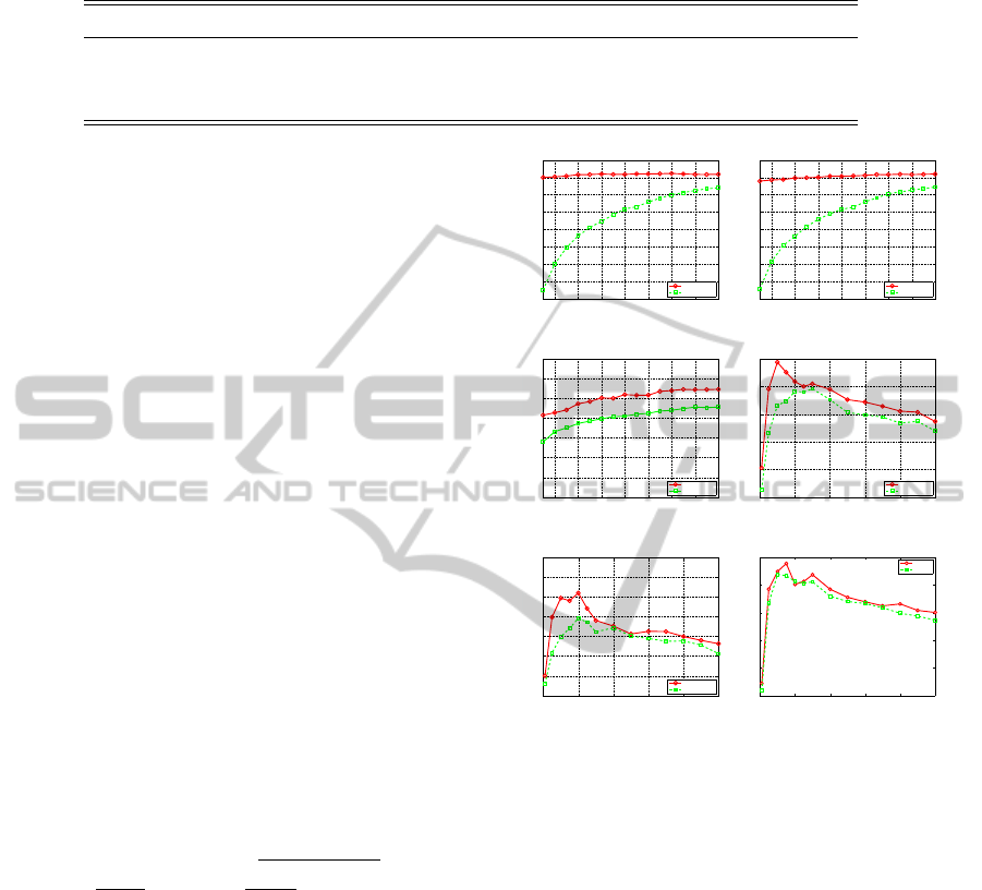
Table 4: Comparison of the macro F

score for different methods. The proposed methods are marked by

∗

, and (U) denotes

unsupervised, (S) supervised.

Method Raw LSI LE USC OLPP CCA MORP MDDM SLE

∗

SUSC

∗

SOLPP

∗

(U/S) N/A (U) (U) (U) (U) (S) (S) (S) (S) (S) (S)

Reuters F

0.890 0.828 0.865 0.870 0.891 0.878 0.900 0.900 0.911 0.912 0.909

k 24,012 1800 1800 1800 1800 1800 1800 1800 1800 1800 1800

EPPI F

0.332 0.387 0.355 0.346 0.424 0.390 0.394 0.385 0.394 0.410 0.457

k 176,624,316 300 100 200 150 500 500 200 100 100 100

between the projected features and the labels, respec-

tively, and MORP minimizes the reconstruction error

of both features and labels.

To obtain the feature-based adjacency graph, two

types of KNN-graph were used, one with the Gaus-

sian kernel weight and the other with constant binary

weight, which were also used as W

to obtain our

multi-label graph. All the model parameters, includ-

ing the number of KNNs, the regularization param-

eter α of out-of-sample extension 2, the parameter

β to control the number of prototypes, the number

of lower-dimensional embeddings k, the degree pa-

rameter θ, and the width parameters of the Gaussian

kernels, were tuned by grid search, using the valida-

tion set for the Reuters data and 3-fold-cross valida-

tion with the training set for the EEP data. To re-

duce the computational complexity of the DR proce-

dure caused by large-scale features, the Euclidean dis-

tance was employed to compute the prototype-based

relation features for the Reuters data, while, the inner-

product for the EEP data.

As support vector machines (SVMs) have shown

success in text categorization (Bennett and Nguyen,

2009), a linear SVM was employed to obtain the

multi-label classiﬁcation performance of different

types of embeddings. The macro average of the F

scores of all classes is computed for performance

evaluation and comparison. For each category, the

score is computed by F

2Precision×Recall

Precision+Recall

, where

Precision =

TP+FP

, Recall =

TP+FN

, TP denotes true

positive, TN denotes true negative, FP denotes false

positive and FN denotes false negative.

4.2 Results and Analysis

Different types of multi-label graph in Section 3.1

were tried for SLE, SUSC and SOLPP, of which per-

formance varies from 0.902 to 0.912 for the Reuters

data, and from 0.387 to 0.457 for the EEP data. It

is observed that the best performance was mostly

achieved with W

deﬁned by the KNN-graph with

the Gaussian kernel weight, and W

computed from

the projected label vectors. We compare our SLE,

SUSC and SOLPP using this best performing multi-

label graph with LE, USC and OLPP using their best

performing feature-based graph (KNN-graph with the

400 600 800 1000 1200 1400 1600 1800

0.55

0.6

0.65

0.7

0.75

0.8

0.85

0.9

0.95

Fscore

supervised

unsupervised

(a) Reuters: LE.

400 600 800 1000 1200 1400 1600 1800

0.55

0.6

0.65

0.7

0.75

0.8

0.85

0.9

0.95

Fscore

supervised

unsupervised

(b) Reuters: USC.

400 600 800 1000 1200 1400 1600 1800

0.8

0.82

0.84

0.86

0.88

0.9

0.92

Fscore

supervised

unsupervised

0 200 400 600 800 1000

0.2

0.25

0.3

0.35

0.4

Fscore

supervised

unsupervised

(d) EEP: LE.

0 200 400 600 800 1000

0.2

0.25

0.3

0.35

0.4

0.45

0.5

Fscore

supervised

unsupervised

(e) EEP: USC.

0 200 400 600 800 1000

0.2

0.25

0.3

0.35

0.4

0.45

Fscore

SOLPP

OLPP

(f) EEP: OLPP.

Figure 1: Performance with respect to the reduced dimen-

sion k for different methods and datasets.

Gaussian kernel weight), respectively, in Table 2 and

Table 3 for both datasets, as well as Figure 1 for differ-

ent values of the resulting dimensionality of embed-

dings. It can be seen from Table 2, Table 3 and Figure

1, our supervised multi-label graph generate embed-

dings with better discriminating power, as compared

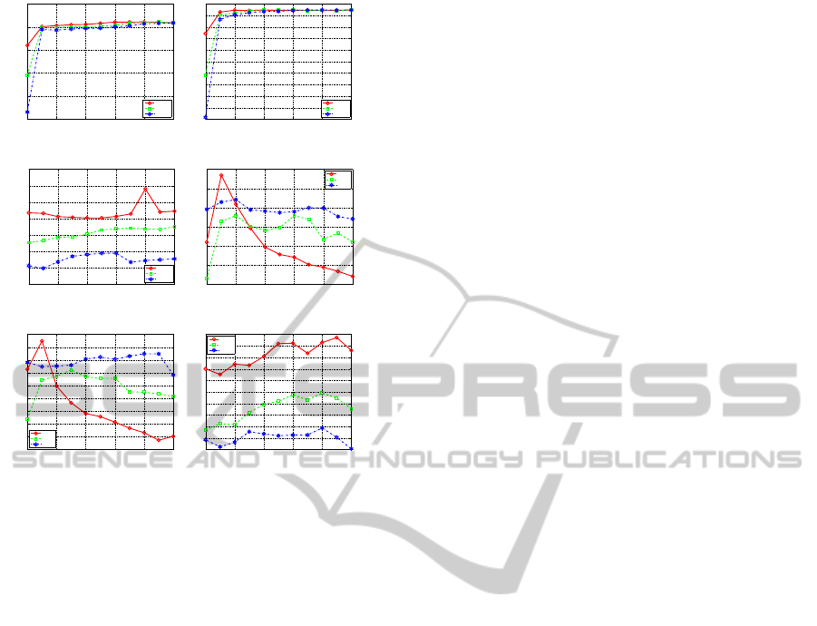
with the unsupervsied feature-based graph. We also

show the impact of the tradeoff between the feature

and label structures in Figure 2, for different meth-

ods and datasets. Different optimal values of θ were

reached for different used values of k. Appropriate

combination of the label and feature information can

improve the performance obtained by solely using

one type of information on its own.

We compare the macro F

scores of our proposed

supervised DR methods with that of four existing un-

supervised DR methods and three existing supervised

DR methods, as well as that of the original features,

denoted as raw features, without applying any DR

PROXIMITY-BASED GRAPH EMBEDDINGS FOR MULTI-LABEL CLASSIFICATION

0 0.2 0.4 0.6 0.8 1

0.7

0.75

0.8

0.85

0.9

0.95

Fscore

k=1800

k=1000

k=600

(a) Reuters: LE.

0 0.2 0.4 0.6 0.8 1

0.72

0.74

0.76

0.78

0.8

0.82

0.84

0.86

0.88

0.9

0.92

Fscore

k=1800

k=1000

k=600

(b) Reuters: USC.

0 0.2 0.4 0.6 0.8 1

0.88

0.885

0.89

0.895

0.9

0.905

0.91

0.915

Fscore

k=1800

k=1000

k=600

0 0.2 0.4 0.6 0.8 1

0.3

0.32

0.34

0.36

0.38

0.4

Fscore

k=150

k=50

k=800

(d) EEP: LE.

0 0.2 0.4 0.6 0.8 1

0.24

0.26

0.28

0.3

0.32

0.34

0.36

0.38

0.4

0.42

Fscore

k=200

k=50

k=800

(e) EEP: USC.

0 0.2 0.4 0.6 0.8 1

0.36

0.37

0.38

0.39

0.4

0.41

0.42

0.43

0.44

0.45

0.46

Fscoe

k=100

k= 50

k= 800

(f) EEP: OLPP.

Figure 2: Impact of the tradeoff between the feature and

label structures controlled by θ, for different methods.

method in Table 4. The original CCA and MORP

both impose the orthogonality condition on the em-

beddings. It is noticed in the experiments the original

CCA and MORP performed unsatisfactorily for both

datasets. However, by imposing the orthogonality

condition on the projections instead, the performance

has been greatly improved, which is reported in Table

4. The results show that most supervised DRmethods

perform better than the unsupervised ones in terms

of classiﬁcation performance. Our proposed meth-

ods provides the highest classiﬁcation performance

for both datasets (see Table 4).

We also show the show the reduction of computa-

tional cost using the prototype-based relation features,

as compared with the original features. To compute

the embeddings based on Eq. (3) or Eq. (5) for the

EEP data using the original features, one needs to de-

compose or compute the inverse of a 176, 624, 316 ×

176, 624, 316 matrix. This makes it impossible to col-

lect the classiﬁcation results in a reasonable time. For

the Reuters data, although with comparatively smaller

size of features, it still took long time (more than

7,000 Sec. using MATlAB with computer of 2.8G

CPU and 4.0 GB Memory) to obtain results using the

original features. By using the prototype-based re-

lation features, the computing time of these methods

was greatly reduced to less than 400 Sec. using MAT-

LAB with the same computer, for both datasets.

5 CONCLUSIONS

In this paper, we have developed algorithms for su-

pervised generation of low-dimensional embeddings

with good discriminating ability to facilitate multi-

label classiﬁcation. This is achieved by modelling

the proximity structure between samples with a multi-

label graph constructed from both feature and multi-

label information. Working in either a binary label

space or a projected real label space, different simi-

larity measures have been used to compute the weight

values of the multi-label graph. By employing the

weighted linear combination of the feature-based and

label-based adjacency graphs, the tradeoff between

the category and feature structures can be adjusted

with a degree parameter. To further reduce the com-

putational cost for classiﬁcation with a large number

of input features, we seek the optimal projections in

a prototype-based relation feature space, instead of

the original feature space. By incorporating the la-

bel information into the construction of the adjacency

graph, performance of LE, USC, and OLPP has been

improved by 2% to 5% for the Reuters data, and by

7% to 18% for the EEP data. Our current method

is applicable to discrete output value (classes). Re-

search on how to extend this to supervised learning

task with continuous output values, such as regres-

sion, is in procedure. The proposed method is a gen-

eral supervised DR approach for multi-label classi-

ﬁcation, which should ﬁnd more applications in IR,

TM, NLP and bioinformatics.

ACKNOWLEDGEMENTS

This research is supported by Biotechnology and Bi-

ological Sciences Research Council, BBSRC project

BB/G013160/1 and the JISC sponsored National Cen-

tre for Text Mining, University of Manchester, UK.

REFERENCES

Barutcuoglu, Z., Schapire, R. E., and Troyanskaya, O. G.

(2006). Hierarchical multi-label prediction of gene

function. Bioinformatics, 22(7):830–836.

Bekkerman, R., Tishby, N., Winter, Y., Guyon, I., and

Elisseeff, A. (2003). Distributional word clusters vs.

words for text categorization. Journal of Machine

Learning Research, 3:1183–1208.

Belkin, M. and Niyogi, P. (2003). Laplacian eigenmaps

for dimensionality reduction and data representation.

Neural Computation, 15(6):1373–1396.

KDIR 2010 - International Conference on Knowledge Discovery and Information Retrieval

Bengio, Y., Paiement, J., Vincent, P., Delalleau, O., Roux,

N. L., and Ouimet, M. (2003). Out-of-sample exten-

sions for LLE, Isomap, MDS, eigenmaps, and spectral

clustering. In Proc. of Neural Information Processing

Systems, NIPS.

Bennett, P. N. and Nguyen, N. (2009). Reﬁned experts:

improving classiﬁcation in large taxonomies. In Proc.

of the 32nd Int’l ACM SIGIR conference on Research

and development in information retrieval.

Blei, D. M., Ng, A. Y., Jordan, M., and Lafferty, J.

(2003). Latent Dirichlet allocation. Journal of Ma-

chine Learning Research, 3:2003.

Cai, D., He, X., and Han, J. (2007a). Spectral regression:

A uniﬁed subspace learning framework for content-

based image retrieval. In Proc. of the ACM Conference

on Multimedia.

Cai, D., He, X., and Han, J. (2007b). Spectral regression

for efﬁcient regularized subspace learning. In Proc. of

the International Conf. on Data Mining, ICDM.

Chan, P. K., Schlag, M. D. F., and Zien, J. Y. (1994). Spec-

tral k-way ratio-cut partitioning and clustering. IEEE

Trans. on Computer-Aided Design of Integrated Cir-

cuits and Systems, 13(9):1088–1096.

Coppersmith, D. and Winograd, S. (1990). Matrix multi-

plication via arithmetic progressions. Journal of Sym-

bolic Computation, 9:251–280.

Deerwester, S., Dumais, S. T., Furnas, G. W., Landauer,

T. K., and Harshman, R. (1990). Indexing by latent

semantic analysis. Journal of the American Society

for Information Science, 41:391–407.

Dhillon, I. S. (2001). Co-clustering documents and words

using bipartite spectral graph partitioning. In Proc. of

the 7th ACM SIGKDD International Conf. on Knowl-

edge discovery and data mining, pages 269–274, San

Francisco, California, US.

Dhillon, I. S., Mallela, S., and Kumar, R. (2003). A division

information-theoretic feature clustering algorithm for

text classiﬁcation. Journal of Machine Learning Re-

search, 3:1265–1287.

Fisher, R. A. (1936). The use of multiple measurements in

taxonomic problems. Annals of Eugenics, 7(2):179–

188.

Gonzalez, T. F. (1985). Clustering to minimize the maxi-

mum intercluster distance. Theoretical Computer Sci-

ence, 38:23–306.

Hardoon, D. R., Szedmak, S. R., and Shawe-taylor, J. R.

(2004). Canonical correlation analysis: An overview

with application to learning methods. Neural Compu-

tation, 16(12):2639 – 2664.

He, X. (2004). Incremental semi-supervised subspace

learning for image retrieval. In Proc. of the ACM Con-

ference on Multimedia.

He, X. and Niyogi, P. (2003). Locality preserving projec-

tions. In Proc. of Neural Information Processing Sys-

tems 16, NIPS.

He, X., Yan, S., Hu, Y., Niyogi, P., and Zhang, H.

(2005). Face recognition using laplacianfaces. IEEE

Trans. on Pattern Analysis and Machine Intelligence,

27(3):328–340.

HildII, K. E., Erdogmus, D., Torkkola, K., and Principe,

J. C. (2006). Feature extraction using information-

theoretic learning. IEEE Trans. on Pattern Analysis

and Machine Intelligence, 28(9):1385–1392.

Huang, Y., Chiang, C., Shieh, J., and Grimson, W. (2002).

Prototype optimization for nearest-neighbor classiﬁ-

cation. Pattern Recognition, (6):12371245.

Jolliffe, I. T. (1986). Principal Component Analysis.

Springer-Verlag, New York, NY.

Kim, H., Howland, P., and Parl, H. (2005). Dimension

reduction in text classiﬁcation with support vector

machines. Journal of Machine Learning Research,

6:3753.

Kokiopoulou, E. and Saad, Y. (2007). Orthogonal

neighborhood preserving projections: A projection-

based dimensionality reduction technique. IEEE

Trans. on Pattern Analysis and Machine Intelligence,

29(12):2143–2156.

Kokiopouloua, E. and Saadb, Y. (2009). Enhanced

graph-based dimensionality reduction with repulsion

laplaceans. Pattern Recognition, 42:2392–2402.

Lewis, D. D. (1992). Feature selection and feature extrac-

tion for text categorization. In Proc. of the work-

shop on Speech and Natural Language, pages 212–

217, Harriman, New York.

Li, S., Xia, R., Zong, C., and Huang, C.-R. (2009). A frame-

work of feature selection methods for text categoriza-

tion. In Proc. of the Joint Conf. of the 47th Annual

Meeting of the ACL and the 4th Int’l Joint Conf. on

Natural Language Processing of the AFNLP, pages

692–700, Suntec, Singapore. Association for Compu-

tational Linguistics.

Luxburg, U. (2007). A tutorial on spectral clustering. Statis-

tics and Computing, 17(4).

Mollineda, R. and andE. Vidal, F. F. (2002). An efﬁcient

prototype merging strategy for the condensed 1-nn

rule through class-conditional hierarchical clustering.

Pattern Recognition, (12):27712782.

Pekalska, E. and Duin, R. (2002). Dissimilarity represen-

tations allow for building good classiﬁers. Pattern

Recognition Letters, (8):943–956.

Pekalska, E., Duin, R., and Paclik, P. (2006). Prototype

selection for dissimilarity-based classiﬁers. Pattern

Recognition, (2):189–208.

Roweis, S. T. and Saul, L. K. (2000). Nonlinear dimension-

ality reduction by locally linear embedding. Science,

290(5500):2323–2326.

Shi, J. and Malik, J. (2000). Normalized cuts and image

segmentation. IEEE Trans. on Pattern Analysis and

Machine Intelligence, 22(8):888–905.

Steinwart, I. (2001). On the inﬂuence of the kernel on the

consistency of support vector machines. Journal of

Machine Learning Research, 2:67–93.

Sugiyama, M. (2007). Dimensionality reduction of multi-

modal labeled data by local ﬁsher discriminant analy-

sis. Journal of Machine Learning Research, 8:1027–

1061.

PROXIMITY-BASED GRAPH EMBEDDINGS FOR MULTI-LABEL CLASSIFICATION

Sugiyama, M. (2010). Semi-supervised local ﬁsher discrim-

inant analysis for dimensionality reduction. Machine

Learning, 78(1-2):35–61.

Sun, L., Ji, S., and Ye, J. (2008). Hypergraph spectral

learning for multi-label classiﬁcation. In Proc. of the

14th ACM SIGKDD International Conf. on Knowl-

edge Discovery and Data Mining, pages 668–676, Las

Vegas, Nevada, USA.

Tang, L., Rajan, S., and Narayanan, V. K. (2009). Large

scale multi-label classiﬁcation via metalabeler. In

Proc. of 18th Int’l Conf. on World Wide Web.

Wall, M. E., Andreas, R., and Rocha, L. M. (2003). Sin-

gular value decomposition and principal component

analysis. A Practical Approach to Microarray Data

Analysis, pages 91–109.

Yan, S., Xu, D., Zhang, B., Zhang, H., Yang, Q., and Lin,

S. (2007). Graph embedding and extensions: A gen-

eral framework for dimensionality reduction. IEEE

Trans. on Pattern Analysis and Machine Intelligence,

29(1):40–51.

Yu, J. and Tian, Q. (2006). Learning image manifolds by

semantic subspace projection. In Proc. of the ACM

Conference on Multimedia.

Yu, S., Yu, K., Tresp, V., and Kriegel, H. (2006). Multi-

output regularized feature projection. IEEE Trans.

on Knowledge and Data Eigeneering, 18(12):1600–

1613.

Zhang, W., Xue, X., Sun, Z., Guo, Y., and Lu, H. (2007).

Optimal dimensionality of metric space for classiﬁca-

tion. In Proc. of the 24th International Conf. on ma-

chine learning, ICML, volume 227, pages 1135–1142.

Zhang, Y., Surendran, A. C., Platt, J. C., and Narasimhan,

M. (2008). Learning from multitopic web documents

for contextual advertisement. In Proc. of 14th ACM

SIGKDD Int’l Conf. on Knowledge Discovery and

Data Mining.

Zhang, Y. and Zhou, Z. (2007). Multi-label dimensional-

ity reduction via dependence maximization. In Proc.

of the 23rd National Conf. on Artiﬁcial intelligence,

volume 3, pages 1503–1505, Chicago, Illinois.

KDIR 2010 - International Conference on Knowledge Discovery and Information Retrieval