
FUZZY KEYWORD ONTOLOGY FOR ANNOTATING
AND SEARCHING EVENT REPORTS
Juhani Hirvonen, Teemu Tommila, Antti Pakonen
VTT Systems Reseach, Vuorimiehentie 3, Espoo, Finland
Christer Carlsson, Mario Fedrizzi, Robert Fullér
Institute for Advanced Management Systems Research, Abo Akademi University
ICT House A 4053, 20520 Turku, Finland
Keywords: Fuzzy ontology, Fuzzy partonomy, Fuzzy reasoning schemes, Knowledge mobilisation, Semantic web.
Abstract: This paper defines and applies a fuzzy keyword ontology to annotate and search event reports in a database.
The ontology is developed by superimposing a fuzzy partonomy on fuzzy classifications. The claim is that
fuzzy keywords will help us find event reports even if the event description is incomplete or imprecise and
that this will provide benefits in finding the relevant problem reports. This will save time and costs when
working with queries on large data- and knowledge bases.
1 INTRODUCTION
The following hypothetical situation was selected as
a starting point: A company writes and stores pieces
of knowledge, called "golden nuggets", in the form
of problem reports, models, recommendations, etc.
Nuggets are documents and they can contain data
extracted from the client’s information systems.
While creating a report the expert author annotates it
with suitable keywords. The internal structure of the
document can thus be ignored, and the problem
scales down to the definition of fuzzy keyword on-
tology.
A knowledge base of golden nuggets of different
types is a generic approach applied by many organi-
sations, for example in incident reporting and elec-
tronic diaries. While trying to preserve some general
applicability, our paper takes a narrower viewpoint
to the topic by assuming that the users are supposed
to be experts so that the meaning of the keywords
will be familiar to them.
The main goals of the paper are (i) to develop
fuzzy keyword ontology for an industrial applica-
tion; (ii) to show that fuzzy ontology will create
effective keyword combinations for database que-
ries; (iii) to introduce a tool (KnowMob) that imple-
ments (i) and (ii): The theory and methods we intro-
duce in this paper implement a new concept called
knowledge mobilisation (cf. Carlsson et al (2010
a,b); Romero (2008)). Knowledge mobilisation
represents a change of paradigm in the creation,
building, handling and distribution of knowledge.
We will show that this differs from the classical
large, complete ontology approach. We will use
fuzzy sets as a basis. This will allow imprecise que-
ries, repeated iterations and supports for learning to
understand problems which are not sufficiently un-
derstood from the beginning. Similar approaches
have been worked out by Calegari and Ciucci (2006,
2010), Lee et al (2005), and Parry (2006) but our
project is one of the first to work out the methods
and the theory for actual industry applications.
2 KEYWORD CATEGORIES
We identified the most important entities used in
searching problem reports that are relevant for de-
scribing problems in a specific engineering context
which in this case is paper making process. We
defined keyword types that are almost independent
of each other. The goal was to characterise problem
situations by a combination of events, systems and
functions affected, materials involved, and process
variables. The goal was to reduce the amount of
251
Hirvonen J., Tommila T., Pakonen A., Carlsson C., Fedrizzi M. and Fullér R..
FUZZY KEYWORD ONTOLOGY FOR ANNOTATING AND SEARCHING EVENT REPORTS .
DOI: 10.5220/0003091002510256
In Proceedings of the International Conference on Knowledge Engineering and Ontology Development (KEOD-2010), pages 251-256
ISBN: 978-989-8425-29-4
Copyright
c
2010 SCITEPRESS (Science and Technology Publications, Lda.)
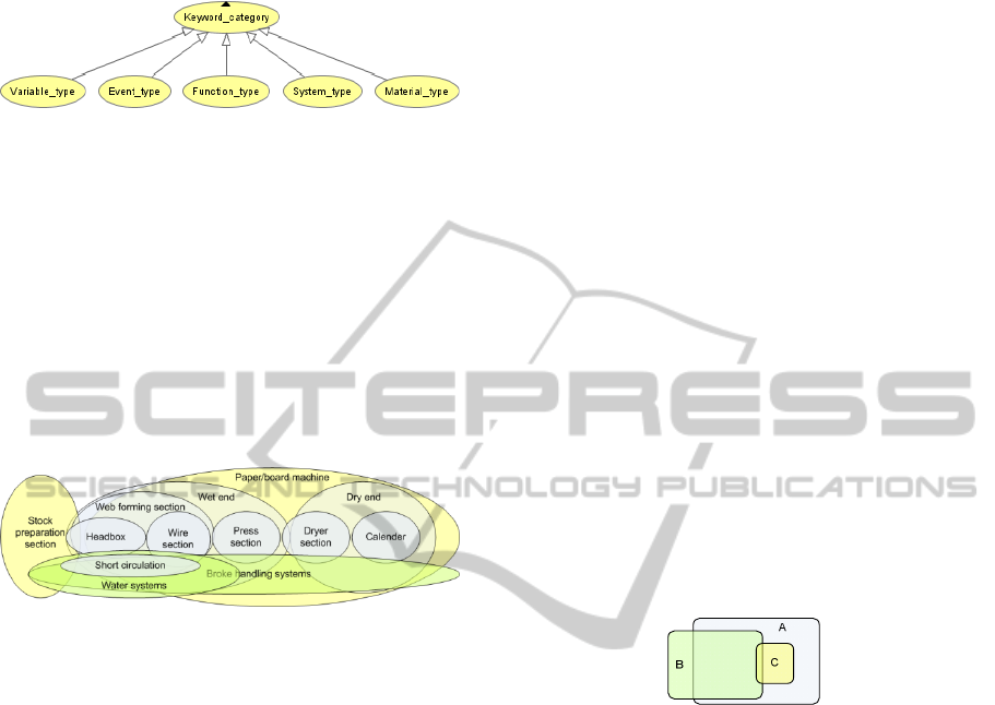
keywords. These adopted keyword categories are
shown in Figure 1.
Figure 1: Keyword categories.
A system is considered to be a real-world entity that
is designed and built for a purpose. Systems consist
e.g. of buildings, mechanical and electrical equip-
ment, software and people. The Figure 2 below
shows some subsystems of a paper making line and
also demonstrates how the system decomposition
often is imprecise depending on the viewpoint taken,
e.g. if the viewpoint is “retention control” then the
effect of “Dry end” to paper quality is negligible.
This means that the effective size of any part of
paper machine is depended on the viewpoint taken.
Figure 2: A “decomposition” of paper line.
The various activities of a system are called
plant functions. In many cases, a function refers to a
purposeful activity. Functions can also be under-
stood as physical and chemical phenomena.
The term process variable refers to attributes of
plant systems, functions, and substances that charac-
terise their performance or state. Very often variable
is measured but it can have a very qualitative charac-
ter even without a numerical scale.
The term event refers to an “episode” in the op-
eration of the plant. Therefore, an event has a dura-
tion that is usually rather short but can continue for
weeks or even months. Quite often, an event is inter-
esting (i.e. valuable for knowledge management)
because it may be unanticipated and unwanted, i.e. a
problematic situation.
An industrial plant processes and handles mate-
rials and substances that have various chemical and
physical properties and purposes in the production
chain.
3 THE FUZZY KEYWORD
CLASSIFICATION
Keywords can be understood as representatives of
sets of real-world events, systems etc. that overlap
and are related in many ways. This complexity is
formalized in a way that serves our purpose, i.e.
finding relevant information from a knowledge base.
This is why we have instead of strict subsethood
adopted another way which is shown in Figure 3.
The set C is fully included in A but the set B con-
tains elements not included in A. Furthermore B
contains a larger part of elements of A than C. In
this way we want to show that some set C of key-
words is included in another set A of keywords; a
second set B of keywords is partly included in A.
There is another aspect to the overlapping of key-
words – the set B partly covers the set A and the set
A fully covers the set C. With the help of this intui-
tive description of inclusion and coverage (which
will be replaced with a formal description in section
4) we have been able to work out fuzzy keyword
classifications that we will show to be fuzzy key-
word ontology (cf. Carlsson et al (2010a).
We will use these inclusion and coverage rela-
tions to classify all Keyword categories.
Figure 3: Inclusion and coverage.
3.1 Event Types
Figure 4 shows a fragment of the fuzzy hierarchy of
Event_types. At the top level generic Event is classi-
fied into problems, neutral observations and suc-
cesses on the basis of the value of the Event. At
lower levels other items are used to categorise prob-
lems into more concrete Event_types.
The two numbers (not all shown) beside the ar-
rows (also not all shown) indicate the inclusion and
coverage values of the related keywords, e.g. “De-
sign_flaw” is included (with degree) 0.60 in “Sys-
tem_fault” and correspondingly 0.40 in “Func-
tion_failure”. The numbers at the lower part of the
arrow give correspondingly the coverage values, e.g.
“Technical_ problem” covers 0.80, “Operational-
_problem” 0.40, and “Quality_problem” 0.50, etc. of
“Problem” events. As a matter of fact this implies
that these keywords overlap (their sum is > 1.00).
KEOD 2010 - International Conference on Knowledge Engineering and Ontology Development
252
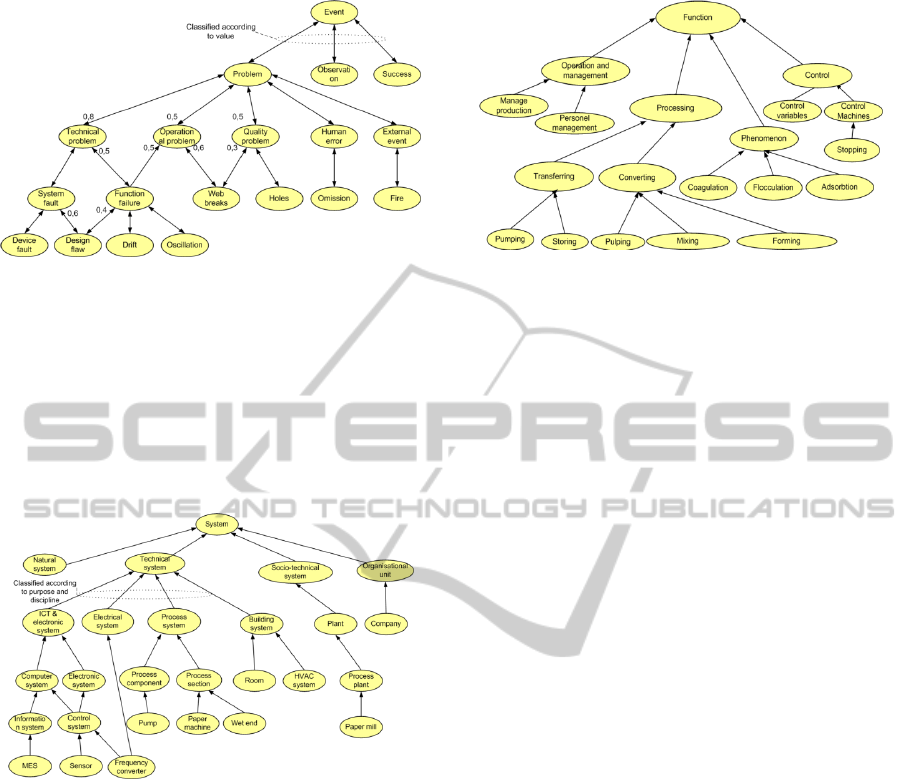
Figure 4: A fragment of the Event_type classification.
3.2 System Types
Figure 5 shows a few examples of generic system
types within an engineering taxonomy that classifies
the parts of a production line in a form of a precise
taxonomy. However, there are several engineering
ontologies and hence we have adopted a fuzzy clas-
sification in the style as used for Event_type.
Figure 5: Classification of System_type, examples.
We are going to need an additional decomposi-
tion of Systems. We call this decomposition parton-
omy. Partonomy fuzzifies the classical whole-part
relationship. For System_type keywords both engi-
neering classification and partonomy are important.
3.3 Function Types
Figure 6 shows some examples of Function_type
keywords and their classification into “Operations
and Management”, “Processing”, “Phenomenon”,
and “Control”. This classification clearly shows how
the independency of categories restricts the amount
of keywords. We do not have separate keywords for
e.g. pH control, retention control, formation control
etc..
Figure 6: Function type keywords, examples.
3.4 Variable Types
Variable names can be added as keywords in order
to say that an event is associated with the variable.
Their values can characterise the situation. Exact
numerical values would not support fuzzy reasoning.
The KnowMob tool (cf. section 5) cannot know
which numerical values should be considered low
and high in a given operational state. The solution is
to let the expert user associate a linguistic value
classification label like “normal”, “high” or “very
low” to a process variable name.
3.5 Dependencies between Categories
In addition to the keyword categories the fuzzy on-
tology must model functional dependencies between
keyword categories. As an example, systems play
various roles in carrying out one or more functions.
These dependencies will be expressed as fuzzy rela-
tions (cf. section 4).
4 FUZZY ONTOLOGY AND
REASONING SCHEMES
We have so far introduced our key concepts and
basic reasoning with an intuitive and “common
sense” approach. In this section we need to become
a bit more precise and introduce more formal defini-
tions of the essential parts of our fuzzy keyword
ontology.
4.1 Fuzzy Ontology
We have as a starting point a basic keyword classifi-
cation which is built on the engineering knowledge
of the paper machine; this keyword classification
can be represented as a directed graph (cf. Figures 4-
6) without loss of generality. Keywords are organ-
ized in five categories <event, system, function,
FUZZY KEYWORD ONTOLOGY FOR ANNOTATING AND SEARCHING EVENT REPORTS
253

variable, material> based on the engineering knowl-
edge; for each category the classification is built on
a specialisation/generalisation relations (i.e. inclu-
sion/coverage relations), i.e. moving to the next
lower level of the directed graph each category
(<event, system, function, variable, material>) is
specified in subclasses (and over sub-sub classes etc
down to specific concepts; i.e. “system elements” if
we follow the “System” category) and moving to the
next higher level of the directed graph sub-classes
(or individual concepts) are generalised to the next
level of sub-classes (or a class).
Keywords are going to be used to quickly find
documents through queries of (very) large databases;
this should be possible by building keyword combi-
nations without following the predefined structure of
the classification but using the relations
We superimpose a partonomy on the keyword
classification, or more precisely a fuzzy partonomy;
this will allow us to find keywords which are partly
the same for a query regardless of where they are
defined in the underlying keyword classification (or
where they are located in the directed graph).
A partonomy that is built on part-of relationships
is a primitive of the formal theory of parthood rela-
tions; parthood relations specify part-of and overlap
within a whole; part-of is reflexive, anti-symmetric
and transitive (the transitivity is sometimes difficult
to justify) and overlap between x and y is defined as
O(x, y) := {z │ z
x and z y} where the symbol
“” now denotes part-of.
The fuzzy keyword classification and partonomy
are built on inclusion and coverage, which are un-
derstood to be relations between fuzzy subsets. The
classifications and part-of relations are collected in
matrices of coverage/inclusion of keywords; the
cells of the matrix are numbers [0, 1] which show
the degree of coverage and inclusion.
A fuzzy ontology is a relation on fuzzy sets, i.e. a
relation associated with a membership function; let
K
i
be a finite fuzzy set of keywords identified with a
level of the directed graph and a category <event,
system, function, variable, material>, hence i = 1,
…, 5; a membership function is a mapping of K
i
x
K
j
on L, a lattice or a partially ordered set; the set of
linguistic labels {negligible, weak, moderate, strong,
perfect} is a lattice which means that a relation be-
tween two sets of keywords can be stated and de-
scribed with a linguistic label.
4.2 Fuzzy Reasoners
We need to find a way to combine linguistic labels
and numbers for the following reasoning schemes so
that we can use them to get numbers for the inclu-
sion/coverage matrix; this can be done in the follow-
ing way (the linguistic labels can be defined accord-
ing to the context; the labels can also be overlap-
ping; cf. Carlsson et al (2010b) for details). Let us
consider a domain of keywords that have
been classified based on some property with real
numbers in [0, 1]; we will consider three fuzzy sub-
sets A, B and C of keywords (similar to K
i
) in the
domain D; we will first work with the fuzzy subsets
A and B. We say that A is a fuzzy subset of B (both
defined in the domain D) and write
(1)
We can then define the two concepts inclusion and
coverage in terms of these fuzzy subsets (as both are
defined in the same domain) by following the
intuitive understanding we have in Figure 3
; it
should be noted that the min-operator is one of a
class of t-norms that can be used to express the
combinations (cf. Carlsson et al (2010b)).
Degree of subsethood (inclusion) of in
,
min
,
/
(2)
Degree of supersethood (coverage)
,
min
,
/
(3)
Now we can combine the two concepts as a
categorisation of the two subsets which can be used
to order the subsets of keywords – for this we have
several possibilities but we can use the following
simple characterisation:
Degree of similarity
,
min
,
/max
,
(4)
It is clear that , ,.
We will get a similar representation of the fuzzy
subset C as it is fully a subset of A (cf. Figure 3).
We can now illustrate these concepts with some
numerical examples; the numbers would be similar
to those used in Figure 4.
Let
0.4,0.6,0.8,0.3 and
0.5,0.4,0.8,0.6.
Then A is almost a subset of B since
for 1,3,4,5 but not quite since
2
KEOD 2010 - International Conference on Knowledge Engineering and Ontology Development
254

2
. The sum of the membership degrees in the
fuzzy set is
∑
0.40.6 0.80.3 2.1
∑
min
,
1.9
Therefore , 0.94, , 0.826,
and , 0.76.
Let next the domain represent the set of keywords
shown in the partial graph in Figure 5.
We can then
find a subset of keywords <Technical_Problem> in
this domain, which has the fuzzy subsets <Sys-
tem_fault> and <Function_failure> of keywords for
which we can work out the inclusion and coverage
relations. In this way we can establish a fuzzy par-
tonomy over the classification of engineering key-
words.
We can then work with the fuzzy partonomy using
so-called approximate reasoning [AR-] schemes to
find and assign summary values to the <Techni-
cal_Problem> subset of keywords to represent how
similar they are to a diagnosis used to identify prob-
lems in the Problem part of the Event partial graph
shown in
Figure 4; As we for the moment do not
have enough empirical data we will use a linear AR-
scheme (which may be too simplified for the con-
text), S_f stands for System_fault, F_f for Func-
tion_failure and T_P for Technical_Problem); then
the scheme would be something like the following:
If S_f is negligible and F_f is negligible then T_P is
negligible
If S_f is weak
and F_f is weak then T_P is weak
If S_f is moderate and F_f is moderate then T_P is
moderate
If S_f is strong
and F_f is strong then T_P is strong
If S_f is perfect
and F_f is perfect then T_P is perfect
If we now denote inclusion with [inc] and cover-
age with [cov] then we should write the ASR-
scheme in the following way using (3) and (4):
If [inc] S_f is <negligible, weak, moderate, strong,
perfect> and [inc] F_f is <negligible, weak, moderate,
strong
, perfect> then T_P is min ([inc] S_f, [inc] F_f)
If [cov] S_f is <negligible
, weak, moderate, strong,
perfect
> and [cov] F_f is <negligible, weak, moderate,
strong, perfect> then T_P is max ([cov] S_f, [cov] F_f)
Then we will have that,
[sim] T_P is = min ([inc] S_f, [inc] F_f)/ max ([cov]
S_f, [cov] F_f)
which now shows how similar (or “good”) T_P is
for identifying the problem at hand.
If we now assume for a moment that we have
collected the necessary data we can insert numbers
and get:
If [inc]S_f is 0.5 and [inc]F_f is 0.4 then T_P is 0.4
If [inc]S_f is 0.6 and [inc]F_f is 0.8 then T_P is 0.6
If [inc]S_f is 0.9
and [inc]F_f is 0.8 then T_P is 0.8
If [inc]S_f is 0.3
and [inc]F_f is 0.5 then T_P is 0.3
In a similar way we can also work out the [cov]
scheme but now we use the max instead of the min.
If [cov]S_f is 0.5 and [cov]F_f is 0.4 then T_P is 0.5
If [cov]S_f is 0.4 and [cov]F_f is 0.3 then T_P is 0.4
If [cov]S_f is 0.6
and [cov]F_f is 0.8 then T_P is 0.8
If [cov]S_f is 0.6
and [cov]F_f is 0.5 then T_P is 0.6
As we found out above (as we are using the
same numbers) then_ 0.94,_
0.826, and _ 0.76.
We should realize that in most cases we do not
have linear AR-schemes and need to have a more
general form for the conclusions. Here the_
is found as the rate of the summed min- and max-
values of the membership values of the keywords in
the fuzzy subsets.
This simple version of a fuzzy reasoner can be
developed into more complete reasoning schemes.
Straccia (2006) has worked out some classes of
reasoners in his fuzzy descriptions logics (fuzzy
DL), which has the added bonus of being part of the
OWL 2.0 standard.
Stoilos et al (2010) worked out fuzzy extensions
to the OWL – going in the opposite direction – and
showed that they will reduce to fuzzy DL.
5 KNOWMOB TOOL
The KnowMob tool implements the fuzzy ontology.
It also implements the fuzzy reasoning.
The KnowMob tool is implemented with Java.
The Protégé ontology editor was used to define and
maintain the fuzzy ontology in OWL format. The
problem solving reports on the chemistry and proc-
ess control of the “wet end” of a paper machine were
collected from our industrial partners. Industrial
experts have assisted in evaluating the results.
5.1 UI for Knowledge Base Query
When browsing the knowledge base for reports that
describe situations similar to the current (problem)
situation, the user first has to describe the situation
at hand. To facilitate an ontology-based query, the
situation must be described using the predefined
keywords. Accordingly, the user interface must help
the user to quickly find the appropriate terms.
FUZZY KEYWORD ONTOLOGY FOR ANNOTATING AND SEARCHING EVENT REPORTS
255
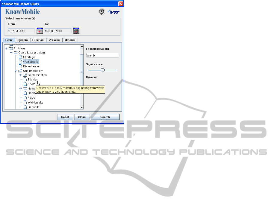
Figure 7: Concept of a user interface for describing the
situation at hand.
The user selects descriptive keywords in categories
such as system (e.g. "paper machine", or "head
box"), function (e.g. "water removal", "hydration"),
event (e.g. "instability" or "drift") and variable (e.g.
"pH", "Brightness"). Because the amount of avail-
able keywords can be staggering, the user is assisted
in finding the particular keyword(s), e.g. by advanc-
ing from more generic keywords to more exact sub-
classes. Since fuzzy ontologies enable multiple in-
heritances, the keyword "Web breaks" can be dis-
covered through different branches, once again mak-
ing it easier to find.
6 CONCLUSIONS
In this paper we showed that we can build a fuzzy
ontology – developed from keyword classification
and a fuzzy partonomy - as a basis for knowledge
mobilization, and we showed that we can form good
keyword combinations to retrieve relevant docu-
ments to deal with process problems in a paper mak-
ing production line.
The aim of the development work was to study
the possibilities that a fuzzy ontology can provide
for knowledge retrieval in the domain of industrial
process plants. We used a fuzzy ontology framework
to describe knowledge related to a paper mill, and
implemented a demo tool for running extended que-
ries against stored reports of knowledge.
The next steps will basically be to generalize
several parts of the results we have shown in this
paper. We need to show that fuzzy ontology – and
the fuzzy description logic that several authors now
have shown that should be used at its core - can be
enhanced with the introduction of AR-schemes to
work with real world data and observations. This
will offer a way to build a connection to the seman-
tic web standards.
ACKNOWLEDGEMENTS
The research project KnowMobile was a joint ven-
ture of IAMSR of Åbo Akademi University, and
VTT Technical Research Centre of Finland; the
project was funded by Tekes (Finnish Funding
Agency for Technology and Innovation) and indus-
trial partners. We are very grateful for the time and
help we got from the industrial partners.
REFERENCES
Calegari, S. and Ciucci, D. (2006): Integrating Fuzzy
Logic in Ontologies. In Proceedings of the 8th Inter-
national Conference on Enterprise Information Sys-
tems, pp. 66-73
Calegari, S. and Ciucci, D. (2010): Granular computing
applied to ontologies. In International Journal of Ap-
proximate Reasoning, 51(4), 391-409
Carlsson, C., Brunelli, M. and Mezei, J. (2010a). Fuzzy
Ontology and Knowledge M obilisation. Turning
Amateurs into Wine Connoisseurs. In Proceedings of
the FUZZ/IEEE 2010 Conference, Barcelona
Carlsson, C., Brunelli, M. and Mezei, J. (2010b). Fuzzy
Ontology and Information Granulation. An Approach
to Knowledge Mobilisation. In IPMU 2010 Proceed-
ings, Dortmund
Lee, C.-S., Jian, Z.-W., Huang, L.-K. (2005): A fuzzy
ontology and its application to news summarization, In
IEEE Transactions on Systems, Man and Cybernetics,
Part B, 35(5), 859-880
Parry, D. (2006): Fuzzy ontologies for information re-
trieval on the WWW. In Fuzzy Logic and the semantic
Web, Vol. 1, Bouchon-Meunier B., Gutierrez Rios J.,
Magdalena, L., Yager R. R. (ed.), Elsevier, Capturing
Intelligence Series
Romero, J. G. (2008): Knowledge Mobilization: Architec-
tures, Models and Applications. PhD Thesis, Universi-
ty of Granada
Stoilos, G., Stamou, G. and Pan, J.Z. (2010): Fuzzy Exten-
sions of OWL: Logical Properties and Reduction to
Fuzzy Description Logics, In Journal of Approximate
Reasoning 51, 656-679
Straccia, U.(2006): A fuzzy description logic for the Se-
mantic Web. In Fuzzy Logic and the Semantic Web,
Vol. 1, E. Sanchez (ed.), Elsevier, Capturing Intelli-
gence Series, 73-90 (Chapter 4)
KEOD 2010 - International Conference on Knowledge Engineering and Ontology Development
256
