A RECEDING HORIZON GENETIC ALGORITHM FOR DYNAMIC
MULTI-TARGET ASSIGNMENT AND TRACKING
A Case Study on the Optimal Positioning of Tug Vessels along the Northern
Norwegian Coast
Robin T. Bye, Siebe B. van Albada and Harald Yndestad
Department of Technology and Nautical Sciences, Ålesund University College, Postboks 1517, N-6025 Ålesund, Norway
Keywords:
Genetic algorithm, Receding horizon predictive control, Resource allocation, Multi-target tracking, Dynamic
environments.
Abstract:
Combining methodologies from cybernetics and artificial intelligence (AI), we present a receding horizon
genetic algorithm (RHGA) for solving the task of dynamic assignment and tracking of multiple targets. We
demonstrate the capabilities of the algorithm by means of a case study on optimal positioning of tugs to reduce
the risk of oil tanker drifting accidents along the northern Norwegian coast. Through simulations we show that
the RHGA performs intelligent target assignment and close target tracking while constantly reevaluating its
suggested solutions based on current and predicted information. We see great potential for further development
and consider our RHGA and problem description a platform for further research.
1 INTRODUCTION
The task of assigning agents to the tracking of multi-
ple targets in a dynamic environment constitutes sev-
eral overlapping challenges. First, there is the prob-
lem of resource allocation: Which agents shall track
which targets? If there is redundancy, that is, there
are more agents than targets, each target can have at
least one agent assigned to it. However, as is com-
monly the case, the number of targets exceeds the
number of agents, meaning that agents are assigned
more than one target. In addition, some targets may
be more important to track than others. This poses a
second problem of tracking, or dynamic positioning,
of agents relative to the targets: How can the agents
collectively move so that net tracking performance is
maximised? Third, tracking performance can be de-
fined as the ability to reduce a cost measure, or func-
tion. How is this cost measure defined? Finally, being
in a dynamic environment, agents need to constantly
reevaluate these problems: How can the agents in-
corporate future changes in the state space, such as
motion of targets and changing dynamics of the sur-
roundings?
In this paper we present a receding horizon ge-
netic algorithm (RHGA) for solving the abovemen-
tioned challenges. To aid the reader and to emphasise
the usefulness of such a method, we undertake a case
study of a real-world example regarding the position-
ing of tug vessels along the coast of northern Norway.
The Norwegian Coastal Administration (NCA) is in
charge of a vessel traffic services (VTS) centre in the
town of Vardø, which in turn administers a number
of tugs. The main task of these tugs is to patrol the
coastline in a manner that reduces the overall risk of
oil spill resulting from drift grounding accidents in-
volving oil tankers.
Oil tankers are required by law to sail along prede-
fined corridors distant to the coastline, meaning that it
is possible to predict a ship’s future position, for ex-
ample by linearly extrapolating its speed along its cor-
ridor. Furthermore, both static (identity, destination,
cargo, etc.) and dynamic (speed, position, heading,
etc.) ship information are constantly being transmit-
ted through the automatic identification system (AIS)
and made available to VTS centres. Together with
weather forecasts and models of factors such as wind
and ocean currents, this information can be used to
predict potential drift trajectories and grounding posi-
tions, for example in the case of a ship losing manoeu-
vrability through steering or propulsion failure (Eide
et al., 2007b). If a tug is close enough, it can inter-
cept the ship’s drift trajectory and tow the ship away
before it runs ashore. Thus, in keeping with the termi-
114
T. Bye R., B. van Albada S. and Yndestad H..
A RECEDING HORIZON GENETIC ALGORITHM FOR DYNAMIC MULTI-TARGET ASSIGNMENT AND TRACKING - A Case Study on the Optimal
Positioning of Tug Vessels along the Northern Norwegian Coast.
DOI: 10.5220/0003087101140125
In Proceedings of the International Conference on Evolutionary Computation (ICEC-2010), pages 114-125
ISBN: 978-989-8425-31-7
Copyright
c
 2010 SCITEPRESS (Science and Technology Publications, Lda.)

nology in the introductory paragraph, the patrol tugs
correspond to agents and the oil tankers’ drift trajec-
tories correspond to target trajectories.
The NCA has developed risk-based decision sup-
port tools based on dynamical risk models that draws
on a vast pool of information (Eide et al., 2007a; Eide
et al., 2007b). Some of this information is static and
certain, such as a ship’s type, its crew, and amount and
type of oil it is carrying. Information about other fac-
tors is uncertain and based on models of wind, ocean
currents, accident frequency and consequences, spill
size and impact, and so on. The decision support tools
are able to aid a human operator at a VTS centre in
commanding tugs by pointing out high-risk positions
that tugs should approach. However, as the number of
tugs and oil tankers grows, the problem of allocating
tugs to several positions quickly becomes non-trivial.
Thus there seems to be a need of a computer program,
or algorithm, that can take the existing models and
decision support tools one step further by calculating
where each tug should move. The calculation may be
based on a number of input variables set by the oper-
ator. For example, particular oil tankers or areas may
be given special priority.
The program should run in real-time, however,
given that it usually takes many hours from the mo-
ment that a ship loses manoeuvrability until it runs
ashore and the relatively slow dynamics of ocean cur-
rents, a moderate update rate suffices.
In the following sections, we will present a sim-
plified version of the tug positioning problem and an
algorithm that solves it by combining receding hori-
zon control (RHC) with a genetic algorithm (GA). We
will show how the RHGA performs in some simulated
scenarios and finally we will discuss our results, lim-
itations to our approach, and future potential.
1.1 Problem Description
To simplify the problem, we will assume that N
o
oil
tankers move in one dimension only up and down
(north and south, say) an oil tanker line of motion y
o
.
This seems reasonable considering that oil tankers are
required to follow predefined straight-line-segmented
corridors. Closer to shore, we assume that N
p
tugs
are moving, or patrolling, up and down a patrol line of
motion y
p
parallel to that of the oil tankers. We ignore
collisions between oil tankers and patrol tugs on their
respective lines of motion. Naturally, we acknowl-
edge that the coastline with its fjords, peninsulas, and
islands does not constitute a straight line, however,
given that tugs should stop drifting ships before they
reach land or danger zones, it seems reasonable to
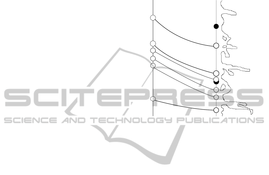
simplify the problem as described. Figure 1 shows
a graphical representation of the problem description.
Next, we assume the availability of an accurate
Oil tanker line
yo
Patrol tugs line
yp
Coast line
Oil tanker
Oil tanker
Oil tanker
Patrol tug
Patrol tug
D
r
i
f
t
t
r
a
j
e
c
t
o
r
y
D
r
i
f
t
t
r
a
j
e
c
t
o
r
y
D
r
i
f
t
t
r
a
j
e
c
t
o
r
y
Cross
point
Cross
point
Cross
point
t = td
t = td
t = td + 1
t = td + 2
t = td + 3
t = td
t = td
t = td + drift time
t = td
t = td + 2 + drift time
t = td+3 + drift time
t = td + 1 + drift time
t = td + drift time
t = td + drift time
Figure 1: Problem description. Oil tankers (white circles)
and patrol tugs (black circles) move in one dimension up
and down (north and south, say) lines y
o
and y
p
, respec-
tively. Predicted drift trajectories starting at some time
t = t
d
with corresponding cross points on the patrol line are
shown as indicated. In addition, dashed circles and lines in-
dicate another three predicted cross points from future drift
trajectories starting at t = t
d
+1, . .. ,t
d
+3 for the oil tanker
in the middle. How should the tugs move in order to best
prevent drift grounding accidents?
model, or set of models, such as those developed by
the NCA and described in Section 1. These mod-
els are able to predict future positions of oil tankers
along y
o
and their corresponding potential drift trajec-
tories given current and predicted information about
ships (e.g., speed and direction) and the environ-
ment (e.g., wind and ocean currents). Specifically,
for an oil tanker positioned at y
o
(t) at time t = t
d
,
the model can predict its future position ˆy
o
(t) for
t = t
d
+ 1, . . . , t
d
+ T
h
, where T
h
is the prediction hori-
zon and we use a discrete-time formulation with a
sampling time of 1 hour. For each position ˆy
o
(t) there
is a corresponding predicted drift trajectory that may
or may not reach the patrol line y
p
at some time in the
future depending on ocean currents, wind conditions,
and other factors. Collecting all predicted drift trajec-
tories for all oil tankers, the model can thus provide
a distribution of cross points where potential drift tra-
jectories cross the patrol line predicted a time T
h
into
the future.
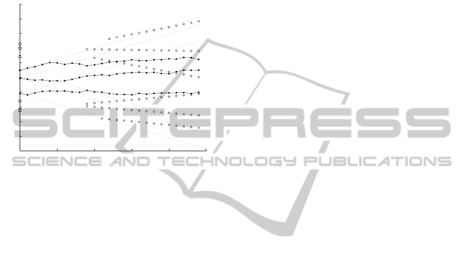
Figure 2 shows an example scenario. Based on
such a distribution, the problem is to calculate trajec-
tories (sequences of patrol points) along y
p
for each
A RECEDING HORIZON GENETIC ALGORITHM FOR DYNAMIC MULTI-TARGET ASSIGNMENT AND
TRACKING - A Case Study on the Optimal Positioning of Tug Vessels along the Northern Norwegian Coast
115

of the patrolling tugs in such a manner as to minimise
the risk that an oil tanker in drift cannot be reached
and saved before grounding. This is a difficult prob-
lem dealing both with resource allocation (which tugs
shall cover which areas) and tracking (how the cover-
age, or tracking of cross points shall be accomplished)
in a dynamic environment.
0 5 10 15 20 25
−100
−80
−60
−40
−20
0
20
40
60
80
100
Time (hours)
Patrol line y
p
or oil tanker line y
o
Figure 2: Example scenario. White squares indicate the
positions of six oil tankers on the oil tanker line y
o
at
t = 0. White circles indicate where predicted drift trajec-
tories cross the patrol line y
p
as a function of time. Black
circles indicate three random patrol trajectories on y
p
for
t = 0, . . . , T
h
, where the prediction horizon is set to T
h
= 24
hours. The regions reachable by the three tugs at full speed
from y
p
(0) are depicted by the dotted lines. All positions
are in arbitrary units.
2 METHOD
2.1 Genetic Algorithm
For the simplest case of a single oil tanker and a sin-
gle tug, classical control theory and mathematics can
provide an analytical solution to solve the problem de-
scribed in Section 1.1, however, this case is mostly
of academic interest. Just by slightly increasing the
number of oil tankers and tugs the problem becomes
exceedingly difficult, cf. Figure 2, which shows three
tugs and three randomly generated patrol trajectories
they may follow in order to track the drift trajecto-
ries of six oil tankers. One possible approach is to
examine a finite number of sets of potential patrol tra-
jectories for the tugs and for each set evaluate some
kind of cost function in order to measure the perfor-
mance of the tugs. There are several methods that
likely can find near-optimal solutions in reasonable
time for this approach, for example variants of Monte
Carlo methods, simulated annealing, ant colony opti-
misation,genetic algorithms (GAs), or other artificial
intelligence (AI) methods. Here, we use a continuous
GA based on a version as described in (Haupt and
Haupt, 2004).
2.1.1 Characteristics of the GA
The GA used in this paper follows the general scheme
used in most GAs (Haupt and Haupt, 2004):
1. Define a cost function and a chromosome encod-
ing and set some GA parameters (mutation, selec-
tion).
2. Generate an initial population of chromosomes.
3. Evaluate a cost for each chromosome.
4. Select mates based on a selection parameter.
5. Perform mating.
6. Perform mutation based on a mutation parameter.
7. If the desired number of iterations or cost level is
reached, stop algorithm and return solution, oth-
erwise, repeat from Step 3.
The selection parameter is in the range 0–1 and
determines how many chromosomes in a population
survives from one iteration to the next. The cost as-
sociated with each chromosome is evaluated and the
chromosomes are given a weighted selection proba-
bility according to their cost, where a smaller cost
results in a greater probability. For a selection pa-
rameter of 0.5, half the population is then randomly
picked, with low cost chromosomes having a greater
chance of being picked, and kept for survival and re-
production. The other chromosomes are discarded to
make room for new offspring.
For mating, the GA uses a combination of an ex-
trapolation method and a crossover method. Informa-
tion from two parent chromosomesare combined with
an extrapolating method to obtain new offspring vari-
able values bracketed by the parents’ variable values.
A single crossover point is used to determine which
parts of the parent chromosomes are used for creating
offspring.
After mating, a fraction of the genes are mu-
tated, which means that the values of these genes
are changed to random numbers within an allowable
range. A mutation rate determines how many genes
are mutated at every iteration. The interested reader
may refer to (Haupt and Haupt, 2004) for further de-
tails on this mating process.
Specific to the problem described in this paper is
the choice of cost function and chromosome encod-
ing. These are described in detail in respective Sec-
tions 2.1.2 and 2.1.3 below.
ICEC 2010 - International Conference on Evolutionary Computation
116

2.1.2 Cost Function
For the results presented in this paper, we define the
cost function as the sum of the distances between all
cross points and the nearest patrol points. The rea-
soning behind this is that if an oil tanker in drift can
be saved by a tug a certain distance away, it is ir-
relevant that other tugs further away can save it at a
later time. Note that "later time" assumes that all tugs
have the same maximum speed.
1
Moreover, as will be
demonstrated in Section 3, choosing this cost function
also yields proper task allocation, as patrol tugs will
tend to spread out and track different groups of cross
points, thus reducing the overall risk of grounding.
We may drop the subscript p for the patrol line y
p
and define y
p
t
as a patrol point on the pth tug’s patrol
trajectory at time t. Similarly, we may define y
c
t
as
a cross point on the cth oil tanker’s drift trajectory at
time t. For N
o
oil tankers and N
p
patrol tugs we can
then define the cost f(t, C
i
) as a function of time t = t
d
and the ith chromosome C
i
:
f(t, C
i
) =
t
d
+T
h
∑
t=t
d
N
o
∑
c=1
min
p∈P
|y
c
t
− y
p
t
| (1)
for P = {1, . . . , N
p
}. C
i
and y
p
t
are defined in the fol-
lowing in Equations 2 and 3, respectively.
2.1.3 Chromosome Encoding
A patrol trajectory for tug p can be obtained from a se-
quence of piecewise constant control inputs (speeds)
u
p
t
in the interval [−1, 1] for points in time t = t
d
+
1, . . . , t
d
+ T
h
. The maximum values at −1 and 1 are
equivalent to tugs going with maximum speed in the
negative or positive y
p
-direction, respectively. This
encoding is generic as it is independent of each tug’s
maximum speed.
To encode N
p
control trajectories as sequences u
p
t
of length T
h
(the prediction horizon) for each patrol
tug p ∈ {1, . . . , N
p
} we use chromosomes C
i
of length
N
p
× T
h
:
C
i
=
h
u
1
1
, . . . , u
1
T
h
, u
2
1
, . . . , u
2
T
h
, . . . , u
N
p
1
, . . . , u
N
p
T
h
i
(2)
That is, each chromosome is a concatenation of N
p
control trajectories, each consisting of T
h
future con-
trol inputs.
The predicted patrol points for tug p are then ob-
tained through linear extrapolation using the differ-
ence equation
y
p
t
= y
p
t−1
+ u
p
t
v
p
m
t
s
, (3)
1
For cases where tugs have different maximum speeds,
one could define arrival time as distance divided by maxi-
mum tug speed and sum the minimum arrival times for each
cross point.
where t
s
= 1 hour is the sampling time, v
p
m
is the max-
imum speed for the pth tug, and t = t
d
+1, . . . , t
d
+T
h
.
2.2 Receding Horizon Control
Given a GA that performs satisfactorily by obtain-
ing patrol trajectories that minimise our desired cost
function, the human operator at a VTS centre could
instruct the tugs to follow the chosen patrol trajecto-
ries in an open-loop manner and perhaps run the al-
gorithm again after some time has passed. A better
choice, however, would be to have the GA run at reg-
ular intervals, constantly incorporating new informa-
tion about oil tanker positions and direction, ocean
currents, weather conditions, and so forth. When
new patrol trajectories have been calculated, the tugs
could replace their respective patrol trajectories with
the new ones. This strategy is equivalent to a receding
horizon control (RHC) scheme, which is interchange-
ably termed model predictive control (MPC) in the
literature.
In RHC, a control strategy, or optimal trajectory,
that minimises some cost function is calculated a pre-
specified duration, or prediction horizon, into the fu-
ture. However only the first portion of the strategy
is implemented before another optimal trajectory is
calculated based on new and predicted information
available. This new trajectory replaces the old one
but again only the first portion is implemented and
the process then repeats.
RHC is currently one of the most popular control
algorithms employed in computer-controlledsystems,
predominantly in the petrochemical industry, but also
increasingly so in electromechanicalcontrol problems
(Goodwin et al., 2001). It can be shown that RHC can
be designed with guaranteed asymptotic closed-loop
stability (Goodwin et al., 2001) and this remarkable
property is perhaps the most important reason for its
popularity.
2.2.1 Constraints
An advantage of using RHC is that constraints can be
handled in the design phase of a control system and
not in some post hoc fashion after the design (Good-
win et al., 2001; Maciejowski, 2002). For the tugs,
an inherent limitation is the maximum speed at which
they can operate. This speed limits the size of the
envelopes in Figure 2 and thus the number of reach-
able cross points. Using RHC combined with the GA
ensures that this limitation is incorporated in the plan-
ning of tug trajectories.
A RECEDING HORIZON GENETIC ALGORITHM FOR DYNAMIC MULTI-TARGET ASSIGNMENT AND
TRACKING - A Case Study on the Optimal Positioning of Tug Vessels along the Northern Norwegian Coast
117

2.2.2 Optimisation
A good choice of initial population for a GA allows
it to quickly (with fewer iterations) find a good solu-
tion. Given that the dynamics of the simulated sce-
nario has not changed "too much," a solution found at
one RHC step should also be a viable solution at the
next RHC step. This is achieved by keeping the best
chromosome at one RHC step, modifying it slightly,
and inserting it into the GA’s initial population at the
next RHC step.
The kept chromosome has to be slightly modified
to accommodate planned trajectories now starting at
the next time instance of the simulation. This involves
a time-shift by discarding the first sample of the tra-
jectories in the best chromosome and adding a new
sample at the end, either with a random value, or, as
we choose to do here, with the same value as the next-
to-last sample.
2.3 Simulation Study
To implement and simulate the scenario presented
above we used the technical computing software
package MATLAB.
2
A number of choices had to be
made about positions, speeds, and directions of ships,
drift rates and directions, the GA and RHC, and gen-
eral settings. After performing some preliminary test-
ing we decided to use the settings described below.
2.3.1 Number of Ships
Based on information provided by NCA staff or af-
filiates and a recent report (Havforskningsinstituttet,
2010), we chose to use N
p
= 3 tugs and N
o
= 6 oil
tankers for our simulations. Whereas these figures are
realistic as of 2009, this situation will change dras-
tically in the near future due to the development of
nearby oil and gas fields (see Section 4.5).
2.3.2 Position of Ships
The initial position of ships at time t = 0 was varied
for each simulation. Specifically, we placed the oil
tankers on the oil tanker line y
o
at positions drawn
randomly from a uniform distribution in the range
[−50, 50] (arbitrary units). Likewise, we placed the
patrol tugs randomly in the same range on the patrol
line y
p
. The reason for doing so was to compare the
performance of the trajectories found by the RHGA
with just keeping the patrol tugs stationary at their ini-
tial positions.
2
MATLAB R2010a, available at http://www.mathworks.
com/.
2.3.3 Velocities of Ships
Each oil tanker was initialised with a random speed
in either the negative (southbound) or positive (north-
bound) y
o
-direction and drawn from a uniform distri-
bution in the range [−1, 1] (arbitrary units). The oil
tankers kept their respective speeds throughout each
simulation.
The patrol tugs were assigned a maximum speed
of 3 (arbitrary units) corresponding to the envelopes
presented previously in Figure 2. This choice was
made to ensure that tugs are much faster than oil
tankers and hence allow for more dynamic task al-
location (change of targets to track) and better track-
ing in our simulations. However, it should be kept in
mind that in the real world, oil tankers have a typical
operating speed of 14–15 knots (Det Norske Veritas,
2009) whereas tugs have a global average maximum
speed of about 12 knots, spanning from 5–26 knots
(Eide et al., 2007b).
3
2.3.4 Drift Trajectories
While we acknowledge that ocean currents and other
factors likely lead to curved drift trajectories perhaps
resembling those in Figure 1, we chose to assume that
any oil tanker in drift will move in a straight line per-
pendicular (directly east) to the patrol line and cross
it after some drift time. That is, if an oil tanker loses
manoeuvrability at y
o
(t
d
) = x, it will cross the patrol
line at y
p
(t
d
+ ∆t) = x after some drift time ∆t.
For each oil tanker we chose a random integer
drawn from a uniform distribution [8, . . . , 12] to be its
drift time and kept it constant throughout each simu-
lation. According to (Eide et al., 2007b), this choice
corresponds to a situation of "fast drift," whereas
"slow drift" means that most tankers will not run
aground within the first 30 hours. Thus, keeping our
drift times in the interval 8–12 hours is a conservative
estimate and in most cases, tugs will have more time
to come to the rescue of a drifting ship.
2.3.5 GA Settings
At every RHC step, we set the GA to perform N
iter
=
100 iterations searching for a solution set of opti-
mal trajectories minimising the cost function given by
Equation 1. A larger number improves the solutions
but it should be kept in mind that each solution set
is replaced at the next RHC step. This next step also
3
A close affiliate to the NCA recently informed us that
typically, in the geographical area of this case study, the
maximum speed of tugs is 15 knots and operating speed of
oil tankers is 10–14 knots.
ICEC 2010 - International Conference on Evolutionary Computation
118

takes advantage of the predictability of the drift tra-
jectories (straight lines) and uses a modified version
of the best chromosome found in the previous RHC
step (see Section 2.2.2).
The population size was set to 10 chromosomes
while the mutation rate was set to 0.1. The selection
parameter was set to 0.5, which implies that the best
half of each population was kept for mating at each
GA interation. These choices gave a good tradeoff
between exploration and exploitation given the other
simulation parameters described previously.
2.3.6 RHC Settings
The GA were used to find optimal trajectories with a
prediction horizonof T
h
= 24 hours for the patrol tugs.
At every RHC step, only the first sample (1 hour)
of these trajectories was executed by the tugs, before
another solution set of trajectories was found by the
GA. This process was repeated for N
RHC
= 26 RHC
steps (that is, each scenario was simulated for t
d
= 0
to t
d
= 25 hours).
2.3.7 General Settings
A total of N
sim
= 20 scenarios (random initial posi-
tions, velocities, and drift times) were simulated. For
each scenario, the optimal costs at each RHC step
were calculated and averaged and stored in vector
f
RHGA
of length N
sim
. Similarly, the costs that would
occur if the patrol tugs would not move from their
initial random positions (static trajectories) were cal-
culated and averaged and stored in a vector f
static
of
length N
sim
.
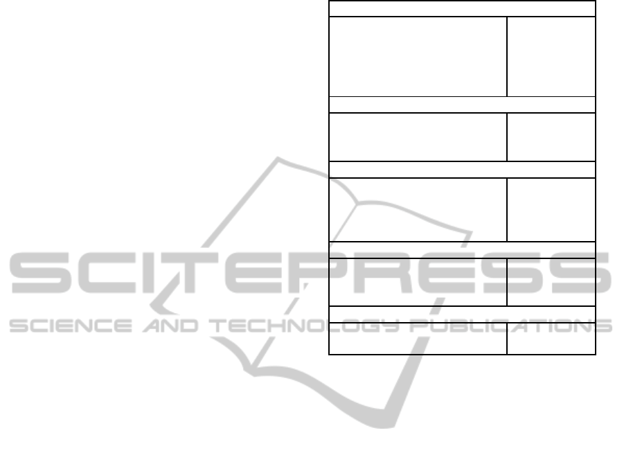
2.3.8 Settings Summary
The simulation settings for patrol tugs and oil tankers
as well as algorithm settings for the GA, the RHC
scheme, and some general settings are summarised in
Table 1.
3 RESULTS
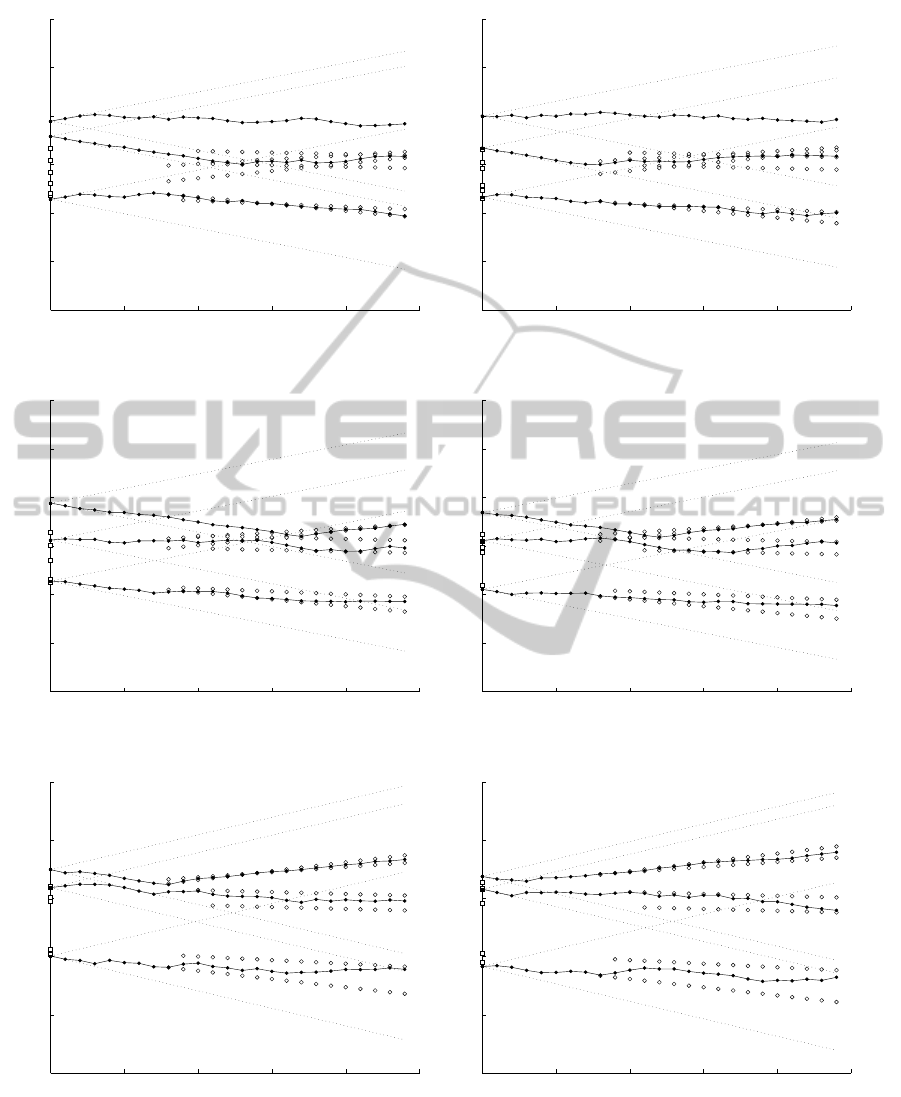
3.1 Simulation example
Figure 3 shows a simulation example using the set-
tings given in Table 1. Initially at drift time t
d
= 0
(Figure 3(a)), three patrol trajectories, each of dura-
tion T
h
= 24 hours into the future, are planned for
the tugs based on the predicted distributions of cross
points, that is, the positions and times where drift tra-
jectories cross the patrol line. The bottom two drift
Table 1: Simulation settings.
Oil tankers
Number of tankers N
o
6
Random initial position [−50, 50]
Random velocity [−1, 1]
Drift direction East
Random drift time ∆t (hours) [8, 9, . . . , 12]
Patrol tugs
Number of tugs N
p
3
Random initial position [−50, 50]
Max velocity ±3
GA settings
Iterations N
iter
100
Population size 10
Mutation rate 0.1
Selection 0.5
RHC settings
Prediction horizon T
h
(hours) 24
Simulation step (hours) 1
Number of steps N
RHC
26
General settings
Number of scenarios N
sim
20
Cost comparison f
RHGA
, f
static
trajectories are close together at around y
p
≈ −40,
thus the RHGA allocates the first and closest tug po-
sitioned at y
1
p
≈ −38 to these two oil tankers by plan-
ning a patrol trajectory that minimises the sum of dis-
tances from these drift trajectories’ cross points to
the nearest patrol points (see Section 2.1.2). Simi-
larly, the remaining four drift trajectories are clustered
around y
p
= 0, and the RHGA allocates the second
and closest tug at y
2
p
≈ 35 to these four oil tankers. Fi-
nally, the third and northmost tug at y
3
p
≈ 48 is not as-
signed any oil tanker and a roughly stationary "don’t
care" trajectory is planned for this tug.
At the next RHC step at t
d
= 1, each tug executes
the first sample (1 hour) of their planned trajectory be-
fore a new set of patrol trajectories, again of duration
T
h
= 24 hours, is planned based on updated informa-
tion about tug and oil tanker positions and predicted
drift trajectories and cross points. This process re-
peats for t
d
= 2, 3, . . . , 25, with the prediction horizon
constantly being shifted one sample, hence the con-
cept of RHC.
Figure 3(b) shows the current positions of oil
tankers and patrol tugs at t
d
= 5. The tugs are allo-
cated the same oil tankers as at t
d
= 0, however, be-
cause some oil tankers are moving north, their pre-
dicted drift trajectories are getting closer to the third
tug at y
3
p
≈ 50. As a result, a change in target alloca-
tion occurs in Figure 3(c), which shows a snapshot of
the situation at t
d
= 10.
A RECEDING HORIZON GENETIC ALGORITHM FOR DYNAMIC MULTI-TARGET ASSIGNMENT AND
TRACKING - A Case Study on the Optimal Positioning of Tug Vessels along the Northern Norwegian Coast
119

0 5 10 15 20 25
−150
−100
−50
0
50
100
150
Time since start: 0 hour(s)
Time (hours)
Patrol line y
p
or oil tanker line y
o
(a) t
d
= 0.
5 10 15 20 25 30
−150
−100
−50
0
50
100
150
Time since start: 5 hour(s)
Time (hours)
Patrol line y
p
or oil tanker line y
o
(b) t
d
= 5.
10 15 20 25 30 35
−150
−100
−50
0
50
100
150
Time since start: 10 hour(s)
Time (hours)
Patrol line y
p
or oil tanker line y
o
(c) t
d
= 10.
15 20 25 30 35 40
−150
−100
−50
0
50
100
150
Time since start: 15 hour(s)
Time (hours)
Patrol line y
p
or oil tanker line y
o
(d) t
d
= 15.
20 25 30 35 40 45
−150
−100
−50
0
50
100
Time since start: 20 hour(s)
Time (hours)
Patrol line y
p
or oil tanker line y
o
(e) t
d
= 20.
25 30 35 40 45 50
−150
−100
−50
0
50
100
Time since start: 25 hour(s)
Time (hours)
Patrol line y
p
or oil tanker line y
o
(f) t
d
= 25.
Figure 3: Example simulation. White squares indicate the positions of six oil tankers on the oil tanker line y
o
at time of drift
t
d
= 0, 5, . . . , 25. White circles indicates where predicted drift trajectories cross the patrol line y
p
as a function of time. Black
circles indicate the current positions and patrol trajectories suggested by the RHGA for three tugs on y
p
for t = t
d
, . . . , t
d
+T
h
,
where T
h
= 24 hours is the prediction horizon. The regions reachable by tugs going at maximum speed from their current
positions y
p
(t
d
) are depicted by the dotted lines. All positions are in arbitrary units.
ICEC 2010 - International Conference on Evolutionary Computation
120

Here, the RHGA plans a trajectory for the third and
northmost tug to begin tracking of the two northmost
drift trajectories (which are so closely positioned that
they are difficult to distinguish), another trajectory is
planned for the second tug to track the two middle
drift trajectories, and the first and southmost tug is
still assigned the two southmost drift trajectories.
Figures 3(d)–3(f) show that this allocation scheme
is maintained for the rest of the simulation: The first
(southmost) tug moves south while tracking the two
southmost drift trajectories, the second (middle) tug is
slowly moving north in order to track the two middle
drift trajectories, and the third (northmost) tug moves
south to track the two northmost drift trajectories.
Notice that in the latter case for the third tug,
the planned trajectories involves moving south at first
to "meet" the northbound drift trajectories and then
move north again while performing close tracking. If
the simulations had been run for t
d
> 25, this would
have become evident in the actually executed position
of the third tug (given that the oil tankers continue
their predicted movements). Similarly, the trajectory
for the second tug begins to tend southward at t
d
= 25
due to the predicted drift trajectories also going south.
Quantitatively, one possible performance measure
is obtained by comparing the cost of applying the
RHGA-generated trajectories to that of static trajec-
tories, that is, keeping each patrol tug p stationary
at its initial position, or y
p
t=0
= y
p
t=1
= . . . = y
p
t=T
h
.
For this simulation example, the overall RHGA cost
was found by summing the costs at t
d
= 0, . . . , 25 and
finding the average cost for each RHC step, which
equalled 463.7 (arbitrary distance units). The static
cost was 1837.4, thus the RHGA improved the static
cost by 74.8 %.
3.2 Main Study
Table 2 summarises the results from the simulation
example above (simulation run 1) and 19 other simu-
lated scenarios based on the settings presented in Ta-
ble 1. For every run, the average cost at each RHC
step t
d
= 0, . . . , 25 is calculated for the static case
(f
static
) and the RHGA case (f
RHGA
). Performance is
measured as the reduction in cost (in percent) from
applying the RHGA instead of the static strategy.
The best performance of the RHGA compared to
static trajectories was obtained in simulation run 12
and showed a cost reduction of 79.0%. The worst per-
formance happened in simulation run 2 and showed a
cost reduction of 26.2%. The mean performance was
a cost reduction of 65.8%.
Comparing the standard deviation of the costs for
static and RHGA trajectories, RHGA showed a reduc-
tion of 70.4%. This is not surprising, considering that
the static strategy can result in low cost trajectories by
chance simply because the drift trajectories roughly
coincide with the initial positions of tugs. Likewise,
the static strategy can lead to some very costly tra-
jectories, because the cross points are far away from
the static tug positions. As a result, the cost for each
simulation scenario will vary greatly depending on
each scenario. The RGHA trajectories, on the other
hand, are constantly being reevaluated at each sample
interval, accommodating both current and predicted
changes to the overall situation. This results in the
RHGA trajectories very effectively tracking the drift
trajectories and reducing the overall cost, which tend
to vary much less than in the static case.
Table 2: Simulation results.
Simulation f
static
f
RHGA
Performance
run (%)
1 1837.4 463.7 74.8
2 1552.2 1145.9 26.2
3 2278.0 675.1 70.4
4 3097.3 1314.0 57.6
5 2822.3 855.8 69.7
6 3929.4 1526.9 61.1
7 2431.7 633.5 73.9
8 2877.1 880.2 69.4
9 3174.7 794.0 75.0
10 1221.5 665.2 45.5
11 3839.0 1113.4 71.0
12 4356.1 914.3 79.0
13 1921.9 818.8 57.4
14 1536.1 583.4 62.0
15 1489.2 869.5 41.6
16 1546.6 575.5 62.8
17 1456.7 457.1 68.6
18 1836.8 445.8 75.7
19 950.8 559.9 41.1
20 3068.0 874.4 71.5
Mean 2361.2 808.3 65.8
Standard dev. 984.7 291.6 70.4
Best run: 12 79.0
Worst run: 2 26.2
3.3 Conclusions
The simulation results show that the RHGA is able
to simultaneously perform multi-target allocation and
tracking in a dynamic environment. The GA calcu-
lates patrol trajectories for allocation and tracking at
regular intervals in time. However, as the environ-
ment changes, an RHC process is employed, where
the GA is constantly used to replan new trajectories
based on current and predicted information.
A RECEDING HORIZON GENETIC ALGORITHM FOR DYNAMIC MULTI-TARGET ASSIGNMENT AND
TRACKING - A Case Study on the Optimal Positioning of Tug Vessels along the Northern Norwegian Coast
121

Employing a cost function related to the distance
from each cross point (where the predicted drift tra-
jectories crosses the patrol line y
p
) to the nearest pre-
dicted patrol trajectory gives good tracking but also
provides task allocation "for free." In short, the patrol
trajectories suggested by the RHGA yield good pre-
vention against possible drift accidents due to taking
the predicted future environment into account.
Nevertheless, this study should be considered a
preliminary study only that perhaps raises more ques-
tions than it answers. These questions will be dis-
cussed in Section 4.
4 DISCUSSION
4.1 Optimisation
Whereas this paper is not concerned with algorithmic
speed optimisation per se, an obvious point of opti-
misation is the choice of initial population in the GA
that must be set at every step of the receding horizon
planning process. Because the dynamics of the prob-
lem scenario is relatively slow-changing (e.g., ocean
currents, wind, or oil tanker speeds and directions),
the initial population should include good individ-
uals, and/or their offspring, from the previous time
step. This will ensure that the GA quickly can tune
in on good solutions, given that the scenario has not
changed too much from the previous time step. For
the simulations presented here, we chose to keep a
modified version of the best chromosome found in
one RHC planning step and put it in the initial pop-
ulation of the next one as described in more detail in
Section 2.2.2.
Moreover, this strategy can be further modified
to reduce the overall number of GA iterations: Af-
ter running a number of iterations at the first RHC
step until a good solution is obtained, only a fraction
of this number of iterations is needed for subsequent
RHC steps. This is because the dynamics are slow-
varying and the GA has "tuned in" to a good solution
space where the previously found solution greatly as-
sists the GA in finding the new, best solution.
Another modification that may speed up algorith-
mic conversion is to include boundary solutions cor-
responding to the trajectory envelope of each tug, that
is, to include solutions in the population correspond-
ing to tugs moving with maximum speed either north
or south. This ensures that "hard-to-find" cross points
far away from the tugs are detected and taken into
considerations.
Finally, it should be kept in mind that only the
best chromosome is transferred at every RHC step.
The other chromosomes are still initialised randomly
(or with some set to boundary solutions as suggested
above). Hence, if novelties have been introduced at
some RHC step, the RHGA will still be able to find
good solutions (albeit requiring more iterations than
for a more static scenario).
4.2 Evaluating Performance
There are several ways to evaluate the performance of
an algorithm. If one is concerned with algorithm con-
vergence speed, one may compare the time or number
of iterations it takes an algorithm to find a solution
with that of other algorithms. We are not particularly
concerned with the rate of convergence of the RHGA
for the case study investigated here. The reason for
this is that the dynamic scenario is relatively slow-
changing and even for a much larger number of sim-
ulated oil tankers and tugs, our algorithm will still be
able to plan trajectories and update them faster than
the real-world time.
To simulate one RHC step with three tugs and six
oil tankers for a particular scenario took about 30 sec-
onds on a MacBook Pro Core 2 Duo 2.53 GHz com-
puter. Increasing the number of oil tankers tenfold to
60 (which might be realistic in the not too distant fu-
ture, see Section 4.5), one RHC step took slightly less
than five minutes. This shows that the RHGA can ac-
commodate much greater complexity than simulated
in this study while staying within the real-time re-
quirement of finishing each RHC step within an hour
of real-time. It also implies that more accurate so-
lutions can be obtained by increasing GA parameters
such as population size and number of iterations at
each RHC step.
Conversely, the small execution time for a RHC
step means that the simulated duration of an RHC
step (1 hour) can be greatly reduced if desired. This
may not be relevant for the study presented here but
implies that systems with much faster dynamics may
take advantage of the RHGA. An example where each
RHC step must be in the range of tenths of seconds or
smaller is real-time control of football-playing robots,
where algorithm speed will most definitely be an is-
sue. For such applications, it is possible to adjust the
GA and RHC settings to obtain small RHC step du-
rations as required. Specifically, one may reduce the
prediction horizon, number of iterations, and popula-
tion size. This may not necessarily degrade perfor-
mance. For example, employing a large prediction
horizon in a football game where it is only possible to
predict actions a short period ahead will not increase
performance, it may even degrade it if it causes each
RHC step to take too long.
ICEC 2010 - International Conference on Evolutionary Computation
122

Another method for measuring performance of an
algorithm is to investigate its ability to reduce a cost
function (or conversely, increase some fitness func-
tion). Using the cost function defined by Equation 1
in Section 2.1.2, we compared the cost of applying
an RHGA strategy with a static strategy where tugs
are kept stationary at their initial random positions.
We found that the RHGA greatly reduces the cost
compared with the static strategy, however, it still re-
mains to compare the RHGA with other intelligent
algorithms for the same problem defined in this pa-
per. Nevertheless, we believe that the results from this
study are very promising and that the RHGA provides
a viable method for solving problems of the kind pre-
sented here.
4.3 Cost Functions
Choosing a suitable cost function is essential for a GA
to be able to solve the problem at hand. While we
believe our choice of cost function in Section 2.1.2 is
a very reasonable one, there are likely other choices
that may be equally, or better, suited to our problem.
One possible cost measure is to count the num-
ber of nonreachable cross points from tug positions
at time t = t
d
to t = t
d
+ T
h
ahead. Nonreachable
points are easily identified as the points that lie out-
side the dotted lines, or envelopes, that depict pa-
trol trajectories of tugs at maximum speed in Fig-
ure 2. Here, one of the southernmost drift trajectory’s
cross points is nonreachable by the southernmost tug
at y
p
(0) ≈ −20. Similarly, seven of the northmost
drift trajectory’s cross points are nonreachable by the
northmost tug at y
p
(0) ≈ 10. This count may then be
repeated for envelopes starting at t = 1, 2, . . . , T
h
− 1
and ending at t = T
h
and finally integrated for all t.
The goal of the GA would then be to select patrol tra-
jectories that minimise the total number of nonreach-
able points, integrated over time.
Preliminary results (not presented in this paper)
using a cost function involving nonreachable cross
points are promising but needs to be investigated fur-
ther. One major drawback is that this method is com-
putationally much more expensive compared to using
the cost function in Section 2.1.2. Another possible
drawback is that the RHGA will not lead to the same
close tracking of predicted drift trajectories as seen in
Figure 3. The reason for this is that the algorithm will
not punish patrol trajectories further away from cross
points than close ones as long as the number of non-
reachable crosspoints does not increase. On the other
hand, this may not be a problem for the case study
presented here. After all, the main goal of the tugs is
to be able to stop a drifting oil tanker from running
aground. Whether this is achieved by close tracking
of predicted drift trajectories or by some other intelli-
gent positioning is not as relevant, although secondary
goals such as minimisation of fuel consumption could
mean that close tracking be given importance.
A potential modification to the cost function in
Section 2.1.2 is to include a term for the control input
in order to punish excessive fuel consumption. For
example, consider Figure 3(a), where the third and
nortmost tug is not assigned any drift trajectory and
as a consequence is given a somewhat "random" os-
cillatory trajectory. Instead of planning such a fuel-
consuming trajectory, including a small input term in
the cost function would ensure that this patrol tug was
simply assigned a stationary trajectory, thus avoiding
unnecessary fuel consumption.
4.4 Other Heuristics
While we have compared the performance of our al-
gorithm with that of a static solution, it could have
been informativeto compareits performancewith that
of an algorithm using some simple heuristic method.
One such method is to let each patrol tug be allocated
the nearest oil tanker not already allocated to another
tug and then let it track that tanker’s drift trajectory.
We have not included any simulations using such a
heuristic in this paper. Nevertheless, we have found
that this method performs well when the numbers of
tugs and tankers are approximately equal but as the
number of tankers increases its performance drops
significantly compared to that of the RHGA. The rea-
son, of course, is that when all tugs have been allo-
cated an oil tanker, they "do not care" about the drift
trajectories of the remaining oil tankers, which in turn
causes evaluations of the cost function to increase.
Another simple heuristic is to spread out the tugs
evenly along the patrol line. Although not simu-
lated, we assume that this method could work rea-
sonably well for very large numbers of tankers since
the tankers’ cross points would then likely be roughly
uniformly distributed along the patrol line (assuming
the tankers not clustering). For a small number of
tankers, on the other hand, this heuristic would not be
able to perform well as cross points would not very
often occur close to the positions of the tugs.
4.5 Simulation Scenarios
There are numerous alternative scenarios that we
could have investigated in this paper. For exam-
ple, we could have lifted some of our restrictions
and incorporated changing drift dynamics (e.g., use
a dynamically-changing vector map for ocean curren-
A RECEDING HORIZON GENETIC ALGORITHM FOR DYNAMIC MULTI-TARGET ASSIGNMENT AND
TRACKING - A Case Study on the Optimal Positioning of Tug Vessels along the Northern Norwegian Coast
123

ts), let patrol tugs have different maximum speeds,
let oil tankers be weighted (e.g., based on their age,
cargo, crew, etc.), and so on. However, most of these
changes will be handled with ease by the RHGA as
they only amount to scaling of variables.
More relevant is the choice of number of ships.
Based on recent information in a governmental re-
port made by the Norwegian Institute of Maritime Re-
search (Havforskningsinstituttet, 2010), our choice of
three tugs and six oil tankers represents a realistic and
typical scenario as of today. Nevertheless, since these
figures are calculated based on measures of yearly
traffic, there will inevitably be days when the num-
ber of oil tankers is greater than six. Moreover, due
the development of large oil and gas fields in the Bar-
ents Sea such as Goliat, Snøhvit, and Shtokman, oil
(and gas) tanker traffic will greatly increase over the
next 10–15 years. As mentioned in Section 4.2, the
RHGA can easily handle the tenfold number of oil
tankers while maintaining real-time requirements and
thus appear well suited for much heavier traffic than
that of today.
We have not simulated cases where drifting actu-
ally occurs nor the situation where a tug becomes un-
available due to refuelling at land or being busy res-
cuing a drifting tanker. Nor have we tried to estimate
how many tugs are necessary to maintain a sufficient
degree of safety for a given number of tankers, which
is highly relevant considering the foreseen increase in
tanker activity. We intend to investigate this further,
in particular in light of other applications where re-
source allocation and deallocation happens even more
frequently.
Finally, it would be of interest to include more re-
alistic two-dimensional (2D) planning for ships and
three-dimensional (3D) planning for aeroplanes or
submersible vehicles. As discussed below, we intend
to continue development of our RHGA to accommo-
date such scenarios.
4.6 Other Applications
In addition to the one-dimensional (1D) problem de-
scribed in this paper, we believe that the RHGA is
suitable for performing multi-target allocation and
tracking in dynamic environments also in 2D and 3D.
This will require modifications to the algorithm and
we have already started this work. A 2D version in
environments with slow dynamics will required lit-
tle modifications, however, for fast dynamics and/or
3D environments, it is likely that the algorithm must
be improved, for example through distributed, paral-
lel control.
Moreover, it could be interesting to combine the
RHGA with so-called boid, or flocking, rules involv-
ing cohesion, separation, and alignment (Reynolds,
1987). In a promising effort, (Luo et al., 2010)
presents a flocking algorithm that modifies the flock-
ing rules by (Reynolds, 1987) and succeeds in multi-
target tracking performed by multiple agents. We
envision that through further development a modi-
fied version of the RHGA could perform equally well
as the algorithm used for the scenarios described by
(Luo et al., 2010).
Furthermore, we note that the problem defini-
tion used in this paper somewhat resembles that of
the RoboFlag Drill described by (Earl and D’andrea,
2007). They describe a scenario where a set of de-
fenders are guarding a circular defence zone against a
set of attackers. The attackers are randomly placed in
an outer circle circumscribing the inner defence zone
and move with constant velocity towards the zone.
The goal of the defenders is to intercept as many of
the incoming attacking trajectories before they reach
the defence zone. It would be of great interest to test
our RHGA for this scenario and compare our results
with those of (Earl and D’andrea, 2007).
4.7 Concluding Remarks
This paper shows that a GA combined with RHC is
able to perform multi-target assignment and track-
ing in dynamically changing environments. Whilst
our results are promising, we consider our study a
preliminary one that needs to be extended for more
scenarios and compared with other intelligent algo-
rithms. Nevertheless, we believe that our problem
description is an interesting and non-trivial challenge
for researchers in the field and welcome alternative
attempts at solving it. Building on the work presented
here, we will continue to refine and extend our RHGA
to other problem scenarios.
Whereas classical control theory and mathemat-
ics can aid in solving assignment and tracking prob-
lems, we see tremendous potential for artificial intel-
ligence (AI) methods in problems where analytical
solutions become non-existent or at least very hard
to find. Such problems may involve nonlinearities
and constraints that AI methods solve with ease. We
firmly believe that the fusion between control systems
theory and AI is the way forward for solving difficult
multi-agent, multi-target problems.
ACKNOWLEDGEMENTS
We wish to thank Jon Leon Ervik at the Norwegian
Coastal Administration and Kjell Røang at Christian
ICEC 2010 - International Conference on Evolutionary Computation
124

Michelsen Research for providing useful information
about oil tanker traffic and positioning of tugs along
the northern Norwegian coast.
REFERENCES
Det Norske Veritas (2009). Rapport Nr. 2009-1016. Re-
visjon Nr. 01. Tiltaksanalyse — Fartsgrenser for skip
som opererer i norske farvann. Technical report, Sjø-
fartsdirektoratet.
Earl, M. G. and D’andrea, R. (2007). A decomposition ap-
proach to multi-vehicle cooperative control. Robotics
and Autonomous Systems, 55:276–291.
Eide, M. S., Øvyind Endresen, Brett, P. O., Ervik, J. L.,
and Kjell Røang (2007a). Intelligent ship traffic mon-
itoring for oil spill prevention: Risk based decision
support building on AIS. Marine Pollution Bulletin,
54:145–148.
Eide, M. S., Øyvind Endresen, Øyvind Breivik, Brude,
O. W., Ellingsen, I. H., Kjell Røang, Hauge, J., and
Brett, P. O. (2007b). Prevention of oil spill from ship-
ping by modelling of dynamic risk. Marine Pollution
Bulletin, 54:1619–1633.
Goodwin, G. C., Graebe, S. F., and Salgado, M. E. (2001).
Control System Design. Prentice Hall, New Jersey.
Haupt, R. L. and Haupt, S. E. (2004). Practical Genetic
Algorithms. Wiley, second edition.
Havforskningsinstituttet (2010). Fisken og havet, særnum-
mer 1a-2010: Det faglige grunnlaget for oppdaterin-
gen av forvaltningsplanen for barentshavet og havom-
rådene utenfor lofoten. Technical report, Institute of
Marine Research (Havforskningsinstituttet).
Luo, X., Li, S., and Guan, X. (2010). Flocking algo-
rithm with multi-target tracking for multi-agent sys-
tems. Pattern Recognition Letters, 31:800–805.
Maciejowski, J. M. (2002). Predictive Control with Con-
straints. Prentice Hall, first edition.
Reynolds, C. W. (1987). Flocks, herds and schools: A
distributed behavioral model. In Computer Graphics
(ACM SIGGRAPH), volume 21, pages 25–34.
A RECEDING HORIZON GENETIC ALGORITHM FOR DYNAMIC MULTI-TARGET ASSIGNMENT AND
TRACKING - A Case Study on the Optimal Positioning of Tug Vessels along the Northern Norwegian Coast
125